Can a Machine Learning Algorithm Predict Your Income Just From Your Demographics?

Ever had a shop assistant walk up and ask, “Can I help you with something?”

Humans can guess instinctively. We observe a person’s clothing, body language, confidence, and even how they speak then guide them toward choices that seem to fit their style or needs. All these are features about a person. We analyze them deduct a budget and style they will be interested in.

But can a machine leaning algo do the same ? Yes, it can. In the above example, the shopkeeper was trying to find if he has seen another individual like me and deduce my wants. We have a similar algorithm. K nearest neighbor. The basic idea behind K-Nearest Neighbors, a simple yet powerful machine learning algorithm that makes predictions based on the behavior of "nearby" data points. Instead of learning complex patterns or weights like other algorithms, KNN looks at the K most similar data points (its "neighbors") and lets them vote to decide the outcome.

TL;DR

Can Your Demographics Reveal Your Paycheck?

Ethical Implications: Bias, Fairness & Inequality

While using demographic data can improve personalization and predictions, it also raises serious ethical concerns that must be addressed.

Bias in Data

Just like human judgment, machine learning can be biased. For example, a shop assistant who regularly sees a certain type of customer may begin to make assumptions based on past patterns, assumptions that may not apply in a different location or context. \n This is exactly what happens in machine learning when models are trained on biased datasets: they inherit patterns that may not generalize well, leading to systematic errors or misinformed decisions.

Fairness

Machine learning models can produce unfair outcomes, often unintentionally. We've seen real-world examples from biased hiring tools to facial recognition systems criticized for unfair treatment of certain groups. \n These outcomes can negatively impact individuals, communities, and society at large.

Inequality

When predictions are linked to pricing or access, they can reinforce existing inequalities. For instance, if a system predicts someone's willingness to pay based on their profile, it might show higher prices to some users creating an unfair experience. \n Take Uber’s surge pricing as an example: while it helps motivate drivers during high-demand times (e.g., during rain or rush hour), it can feel exploitative to riders who have no other choice.

As an example, we can look at

Adult Dataset

• Origin: UCI Machine Learning Repository
• Size: 48,842 instances, 14 attributes
• Ethics: The dataset is publicly available for research and educational purposes.

It contains anonymized census data, and its use complies with ethical standards for open data. The Adult dataset contains demographic information and income labels.

Objective

The main objective is to predict whether a person earns more than $50K/year based on attributes such as age, education, occupation, and hours worked per week.

Algorithm to the solution

k-Nearest Neighbors Algorithm: kNN is a non-parametric, instance-based learning algorithm used for classification and regression. We can use it for classification as well but we will use to predict income based on the attributes at hand.

Euclidean distance

The most common way to measure the distance between two points in space.

A "straight-line" distance between two points. If we use a ruler to measure how far apart two dots are on a piece of paper.

Steps:

• Choose k (here, k=5).
• Compute the Euclidean distance from the query point to all training points.
• Select the k nearest neighbors.
• Assign the class most common among the neighbors.

Assumptions:

• All features contribute equally (hence, normalization is important).

Data import and exploration

import pandas as pd import numpy as np import matplotlib.pyplot as plt import seaborn as sns from sklearn.model_selection import train_test_split, cross_val_score from sklearn.neighbors import KNeighborsClassifier from sklearn.metrics import confusion_matrix, accuracy_score, roc_auc_score, roc_curve, classification_report  # Load dataset url = 'https://archive.ics.uci.edu/ml/machine-learning-databases/adult/adult.data' columns = ['age', 'workclass', 'fnlwgt', 'education', 'education-num', 'marital-status',            'occupation', 'relationship', 'race', 'sex', 'capital-gain', 'capital-loss',            'hours-per-week', 'native-country', 'income'] df = pd.read_csv(url, names=columns, na_values=' ?', skipinitialspace=True)  # Initial exploration print(df.head()) print(df.info()) print(df.describe()) 

output #   Column          Non-Null Count  Dtype  ---  ------          --------------  -----   0   age             32561 non-null  int64   1   workclass       32561 non-null  object  2   fnlwgt          32561 non-null  int64   3   education       32561 non-null  object  4   education-num   32561 non-null  int64   5   marital-status  32561 non-null  object  6   occupation      32561 non-null  object  7   relationship    32561 non-null  object  8   race            32561 non-null  object  9   sex             32561 non-null  object  10  capital-gain    32561 non-null  int64   11  capital-loss    32561 non-null  int64   12  hours-per-week  32561 non-null  int64   13  native-country  32561 non-null  object  14  income          32561 non-null  object 

Feature Descriptions:

• age: The age of the individual (integer).

• workclass: Type of employment (e.g., Private, Self-emp-not-inc, Federal-gov).

• fnlwgt: Final weight, a census-specific numeric value representing the number of people the entry is meant to represent.

• education: Highest level of education attained (e.g., Bachelors, HS-grad, Masters).

• education-num: Numeric representation of education level (e.g., 9 for HS-grad, 13 for Bachelors).

• marital-status: Marital status (e.g., Married-civ-spouse, Never-married, Divorced).

• occupation: Type of job or profession (e.g., Tech-support, Craft-repair, Exec-managerial).

• relationship: Family relationship within the household (e.g., Husband, Wife, Not-in-family).

• race: Race of the individual (e.g., White, Black, Asian-Pac-Islander).

• sex: Gender of the individual (Male or Female).

• capital-gain: Income from investment sources other than wages (integer).

• capital-loss: Losses from investment sources other than wages (integer).

• hours-per-week: Number of hours worked per week (integer).

• native-country: Country of origin (e.g., United-States, Mexico, India).

• income: Target variable; income class (<=50K or >50K per year).

  \

We will drop null values, encode categorical columns and normalize features.

df = df.dropna() df = pd.get_dummies(df, drop_first=True)  from sklearn.preprocessing import StandardScaler scaler = StandardScaler() X = df.drop('income_>50K', axis=1) y = df['income_>50K'] X_scaled = scaler.fit_transform(X)  plt.figure(figsize=(8,4)) sns.histplot(df['age'], bins=30) plt.title('Age Distribution') plt.show()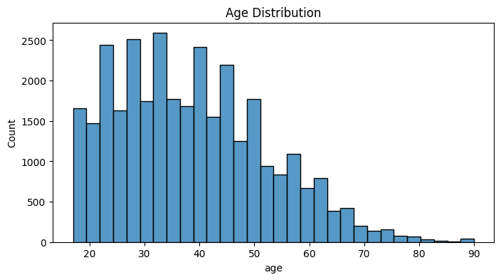 

Age is right skewed. Skewness: 0.56

The age is more concentrated on the prime working years of life which is great. Our dataset might have collected a healthy concentration of working individuals.

Class distribution:

No of people earning more than 50k in the dataset is around 8000. While less than that has a high frequency of around 25000. This is an unbalanced dataset.

sns.countplot(x='income_>50K', data=df) plt.title('Class Distribution') plt.xlabel('Income >50K') plt.ylabel('Count') plt.show()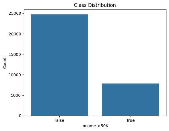 

As always we need train and test data. 80:20 is a healthy split.

| Parameter | Meaning | |----|----| | n_neighbors=5 | The classifier will look at the 5 nearest neighbors (based on distance) to decide how to classify a new data point. This is the "K" in KNN. | | metric='minkowski' | Specifies the distance metric to use. Minkowski is a general form that can represent multiple types of distance (like Euclidean or Manhattan) depending on p. | | p=2 | When p=2, the Minkowski metric becomes Euclidean distance. This is the most common type of distance — the "straight line" distance between two points. |

X_train, X_test, y_train, y_test = train_test_split(X_scaled, y, test_size=0.2, random_state=42) knn = KNeighborsClassifier(n_neighbors=5, metric='minkowski', p=2) knn.fit(X_train, y_train) y_pred = knn.predict(X_test)  print(classification_report(y_test, y_pred))  acc = accuracy_score(y_test, y_pred) print(f'Accuracy: {acc:.2f}')  y_prob = knn.predict_proba(X_test)[:,1] fpr, tpr, thresholds = roc_curve(y_test, y_prob) plt.plot(fpr, tpr) plt.xlabel('False Positive Rate') plt.ylabel('True Positive Rate') plt.title('ROC Curve') plt.show() print(f'ROC-AUC: {roc_auc_score(y_test, y_prob):.2f}')  cm = confusion_matrix(y_test, y_pred) sns.heatmap(cm, annot=True, fmt='d') plt.title('Confusion Matrix') plt.show()  output -->                   precision    recall  f1-score   support         False       0.87      0.90      0.89      4942         True       0.65      0.57      0.61      1571      accuracy                           0.82      6513    macro avg       0.76      0.74      0.75      6513 weighted avg       0.82      0.82      0.82      6513  Accuracy: 0.82 ROC-AUC: 0.84 

The model is much better at identifying people who do not earn more than $50K (high recall and precision for "False") than those who do (lower recall and precision for "True"). This is common in imbalanced datasets. The overall accuracy is good, but the model may miss a significant portion of high-income individuals.

0.82 means that this kNN model correctly predicted the income class for 82% of the individuals in our test dataset. In other words, out of all predictions made, 82% matched the actual labels. This indicates good overall performance.

\ A ROC-AUC score of 0.84 indicates that, on average, there is an 84% chance that the model will rank a randomly chosen positive instance (earns >$50K) higher than a randomly chosen negative instance (does not earn >$50K). This suggests this model performs well in terms of overall classification and is effective at separating the two income classes.

Given a person's demographic information, we can reliably predict whether they earn more than $50K—much like how a human might make an informed guess based on similar details.

Next steps

Deploying the model on AWS SageMaker would demonstrate how insights from a survey can translate into real-world, scalable applications.