Does Progressive Training Improve Neural Network Reasoning Ability?
Table of Links
Abstract and 1. Introduction
1.1 Syllogisms composition
1.2 Hardness of long compositions
1.3 Hardness of global reasoning
1.4 Our contributions
-
Results on the local reasoning barrier
2.1 Defining locality and auto-regressive locality
2.2 Transformers require low locality: formal results
2.3 Agnostic scratchpads cannot break the locality
-
Scratchpads to break the locality
3.1 Educated scratchpad
3.2 Inductive Scratchpads
-
Conclusion, Acknowledgments, and References
A. Further related literature
B. Additional experiments
C. Experiment and implementation details
D. Proof of Theorem 1
E. Comment on Lemma 1
F. Discussion on circuit complexity connections
G. More experiments with ChatGPT
B Additional experiments
B.1 Implications on random graphs
Here, we further discuss the disadvantages of using random graphs as the graph distribution for the implications task. There are two main downsides to using random graphs distribution instead of the cycle task distribution (Definition 1):
\
-
The distance between nodes (i.e., the number of statements to compose) does not scale well with the number of nodes/edges in the graph.
\
-
Whether two nodes are connected or not often correlates with low-complexity patterns such as the degree of the nodes in random graphs, thus, weak learning on random graphs does not necessarily imply that the model has truly learned to find a path between two nodes. In other words, the model may be able to rely on shortcuts instead of solving the composition task.
\ In this section, we provide empirical evidence for both of the claims above.
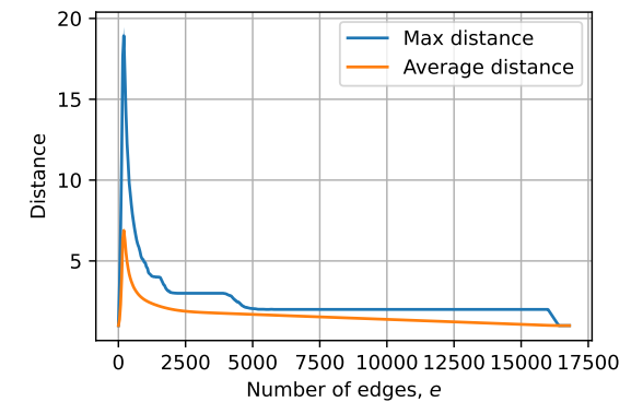
\ First, we consider random graphs with n nodes and a varying number of edges e. For each pair of (n, e), we compute the average of maximum distance and the average of the average distance in random graphs with n nodes and e edges. (We ignore the nodes that are not connected.) The results for n = 128 are presented in Figure 6. It can be seen that the distances in the graphs do not scale well with the number of nodes and edges in the graph. (E.g., compare this to having distance n in the cycle task with 2n nodes/edges.) This is because a high number of edges usually results in a very well-connected graph and a low number of edges leads to mostly isolated edges.
\ Now, we move to the second claim, i.e., the model using low-complexity patterns and correlations. As an example, we take random graphs with 24 nodes and 24 edges. In order to have a balanced dataset with samples of mixed difficulties, we create the dataset as follows. We first sample a random graph with 24 nodes and edges. Then with probability 0.5 we select two nodes that are not in the same connected component (label 0) and with probability 0.5 we choose a distance d ∈ {1, 2, 3, 4} uniformly and we choose two nodes
\ 
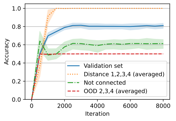
\ that have distance d (if the graph does not have any two nodes with distance d, we sample another random graph). As a result, our dataset is balanced and 12.5% of the samples have distance d for d ∈ {1, 2, 3, 4}. We trained our model on this dataset and we observed that the model reaches an average accuracy of roughly 80%. The results are shown in Figure 7. More precisely, we observed that the model has perfect accuracy when the two nodes are connected (there is a path), and has around 60% accuracy when the two nodes are not connected (the nodes are not in one connected component). In other words, the default behavior of the model is to say that the nodes are connected and the model can also detect that two nodes are not connected in 60% of the cases.
\ To further test whether the model is truly understanding that the two nodes are not connected or it is only relying on low-complexity correlations, we designed new data distributions and assessed the model’s behavior on these new distributions. The samples in the new distributions also have 24 nodes and edges so the model does not have a length generalization problem. More specifically, for i ∈ {2, 3, 4}, we designed distribution OOD i such that each dataset is balanced and for each sample, the two nodes are either in a cycle of size 2i with distance i or they are in two disjoint cycles of size i. All the other nodes are also in different cycles.[11] Note that these distributions are motivated by the cycle task. For example, it is not possible for the model to merely rely on the degree of the nodes. However, if the model uses the correct algorithm (i.e., tries to find a path) then the number of reasoning steps (e.g., length of the BFS/DFS search) is i as the distance between the nodes is i when they are connected and otherwise they are connected exactly to i − 1 other nodes. As it can be seen in Figure 7, the model has 50% (random) accuracy on these distributions meaning that it is not really checking whether there is a path between two nodes or not, even for simple examples in OOD 2 supporting that the model is relying on correlations rather than finding a path. (In particular, the model always outputs connected on these OOD datasets.)
\ We tried to further understand the behavior of this model. By sampling, we computed that one can get an accuracy of around 82% on in-distribution samples just by outputting not-connected if the out-degree of the source query node or the in-degree of the destination query node is zero and connected otherwise. Further, we noticed that this predictor has a high correlation with the output of the model. In particular, in almost all of the cases that the model predicts not-connected, the source’s out-degree or the destination’s in-degree is zero. (The model may still misclassify some of such samples depending on the random seed.) The latter shows that the model is indeed relying on the degrees of the query nodes as a shortcut.
\ 
\
B.2 Change of distribution and curriculum learning
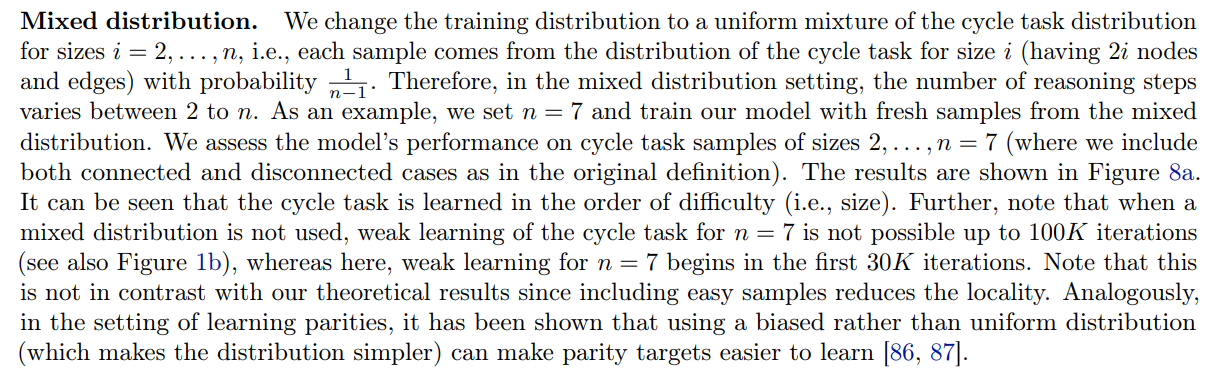
We have defined the cycle task such that all samples in the dataset have the same difficulty. More specifically, if the two nodes are connected their distance is n and if they are not connected they are each in a cycle with n vertices. Thus, it is a natural question to ask what would happen if the training distribution included samples of varying difficulties. To investigate the answer to this question, we use a distribution with samples of mixed difficulties for the training. Furthermore, we try curriculum learning [85] by increasing the samples’ difficulty throughout the training.
\ 
\ Curriculum learning. Next, we try curriculum learning, i.e., we give samples in the order of difficulty (size in the cycle task) to the model during training. We consider two settings: (1) a setting in which the model has to fit samples of all difficulties and (2) a setting in which the model is allowed to forget easier samples. In other words, in the first setting, we want the model to fit cycle task samples of sizes 2, . . . , n while in the second setting, we only care about fitting samples of size n. We start with the first setting which is closer to
\ 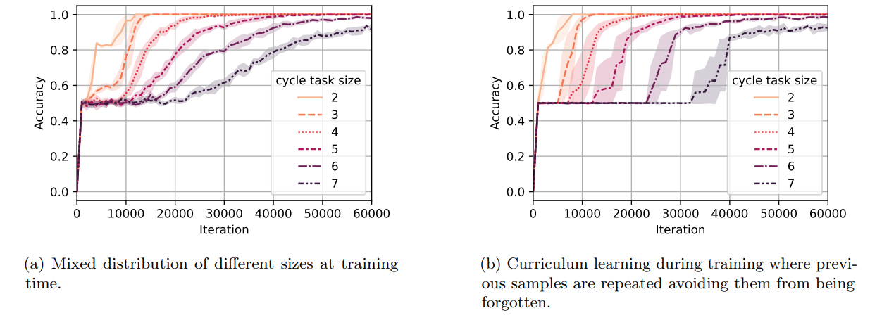
\ the notion of mixed distribution above. We consider distributions D2, . . . , Dn such that distribution Di is a uniform mixture of cycle task samples of sizes 2, 3, . . . , i (e.g., Dn is the mixed distribution used for the mixed distribution setting of Figure 8a). We start training on D2 and we change training distribution from Di to Di+1 when reaching a 95% accuracy on Di . The results for this curriculum setting are provided in Figure 8b. Comparing this curriculum setting to the use of mixed distribution without curriculum (Figure 8a), we can see that curriculum learning helps the model reach a high (e.g., 80%) accuracy slightly faster. Nevertheless, note that weak learning starts earlier in the mixed distribution setting, as the model is trained on samples of all difficulties from the beginning. The general observation that beyond using a mixed distribution, curriculum is helpful for learning has been previously shown both theoretically [88] and empirically [89].
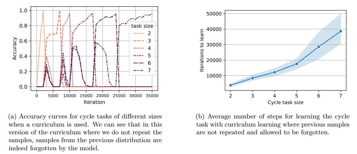
\ Now, we move to the second setting where we allow easier samples to be forgotten. More precisely, we consider distributions D2, . . . , Dn such that distribution Di is the distribution of samples of the cycle task of size i (i.e., 2i nodes and edges). Similarly, we start training on D2 and we go from Di to Di+1 when reaching a 95% accuracy on Di . We present the accuracy curves for a single random seed in Figure 9a. We further provide the average number of iterations required to reach 0.95% accuracy for the cycle task of different sizes in Figure 9b. It can be seen that the time complexity for this variant of the curriculum method is lower than the former curriculum method at the cost of forgetting samples of smaller sizes.
\ In sum, using distributions with samples of a mixed difficulty and also curriculum learning can reduce the learning complexity. (E.g., they made cycle task of size 7 learnable). Nevertheless, the scratchpad approaches are still significantly more efficient (see Figure 4a).
B.3 Learning parities with scratchpad
\ 
B.4 Length generalization for the parity task
\ 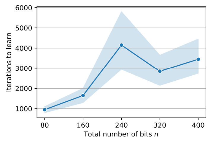
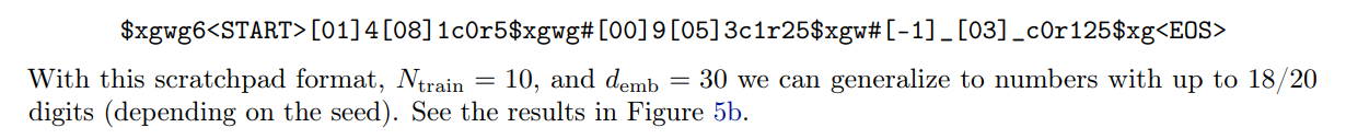
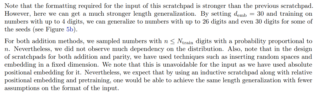
B.5 Length generalization for the addition task
\ In other words, at each iteration, we shift the ans to the right (and lose the rightmost token). Instead, we concatenate the ith digit of the summation to it from the left. So in general, the model has to increase the pointers in the scratchpad, read their corresponding values, and do one summation using them (and the carry in the previous state) at each reasoning step. The scratchpad ends when both numbers are finished. Note that the answer is always the string to the left of $ at the end of the text. Thus, the completed scratchpad for our example (where input is 94+3__1=) can be given by
\ 
\ 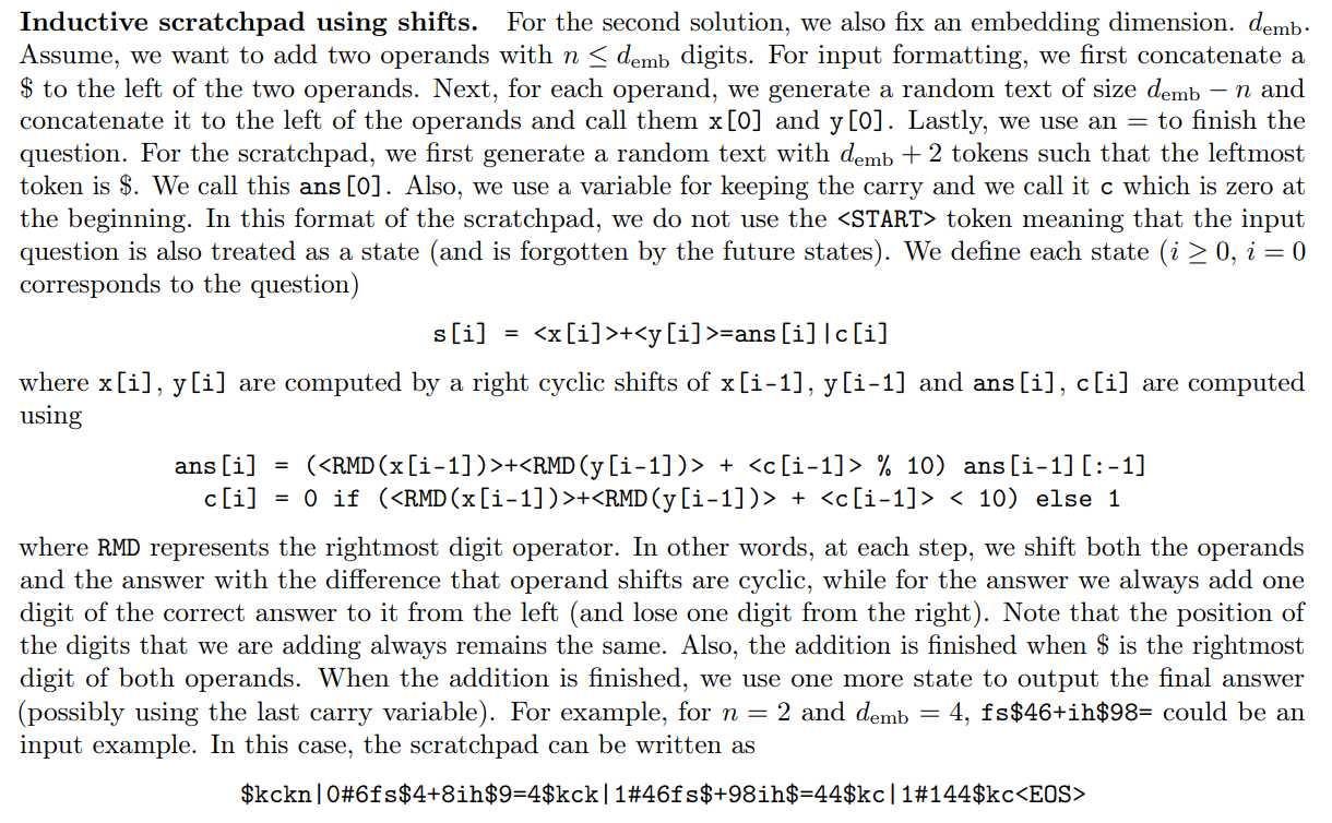
\ In the example above one can note that some part of the s[0] is in the question and some part of it is in the scratchpad.
\ 
\
:::info Authors:
(1) Emmanuel Abbe, Apple and EPFL;
(2) Samy Bengio, Apple;
(3) Aryo Lotf, EPFL;
(4) Colin Sandon, EPFL;
(5) Omid Saremi, Apple.
:::
:::info This paper is available on arxiv under CC BY 4.0 license.
:::
[11] For example, for i = 3, distribution OOD 3 consists of graphs with 4 cycles of size 6 where the nodes are in a single cycle and their distance is 3 and graphs with 5 cycles of sizes 3,3,6,6,6 where the query nodes are in the two cycles of size 3.


You May Also Like

Why Is MemeCore Up 20% Today?

Telegram steps in as Toncoin validator – Can $191M staking drive TON’s rally?