From vx, vy to δ and a: The Math Behind Smarter Self‑Driving Predictions
Table of Links
Abstract and I. Introduction
II. Related Work
III. Kinematics of Traffic Agents
IV. Methodology
V. Results
VI. Discussion and Conclusion, and References
VII. Appendix
III. KINEMATICS OF TRAFFIC AGENTS
Our method borrows concepts from simulation and kinematics. In a traffic simulation, each vehicle holds some sort of state consisting of position along the global x-axis x, position along the global y-axis y, velocity v, and heading θ. This state is propagated forward in time via a kinematic model describing the constraints of movement with respect to some input acceleration a and steering angle δ actions. The Bicycle Model, both classical and popularly utilized in path planning for robots, describes the kinematic dynamics of a wheeled agent given its length L:
\ 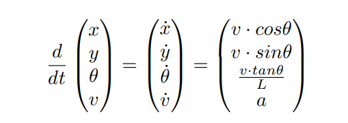
\ We refer to this model throughout this paper to derive the relationship between predicted distributions of kinematic variables and the corresponding distributions of positions x and y for the objective trajectory prediction task.
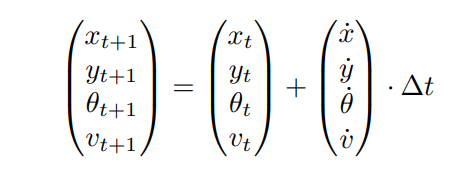
\ We use Euler time integration in forward simulation of the kinematic model to obtain future positions. As we will show later, explicit Euler time integration is simple for handling Gaussian distributions, despite being less precise than higher-order methods like Runge-Kutta. Furthermore, higher-order methods are also difficult to implement in a parallelizable and differentiable fashion, which would add additional overhead as a tradeoff for better accuracy. An agent’s state is propagated forward from timestep t to t + 1 with the following, given a timestep interval ∆t:
\ 
\
IV. METHODOLOGY
A. Probabilistic Trajectory Forecasting
Trajectory forecasting is a popular task in autonomous systems where the objective is to predict the future trajectory of multiple agents for T total future timesteps, given a short trajectory history. Recently, state-of-the-art methods [29], [30], [31], [7] utilize Gaussian Mixture Models (GMMs) to model the distribution of potential future trajectories, given some intention waypoint or destination of the agent and various extracted agent or map features. Each method utilizes GMMs slightly differently, however, all methods use GMMs to model the distribution of future agent trajectories. We apply a kinematic prior to the GMM head directly—thus, our method is agnostic to the design of the learning framework. Instead of predicting a future trajectory deterministically, current works instead predict a mixture of Gaussian components (µx, µy, σx, σy, ρ) describing the mean µ and standard deviation σ of x and y, in addition to a correlation coefficient ρ and Gaussian component probability p. The standard deviation terms, σx and σy, along with correlation coefficient ρ, parameterize the covariance matrix of a Gaussian centered around µx and µy.
\ Ultimately, the prediction objective is, for each timestep, to maximize the log-likelihood of the ground truth trajectory waypoint (x, y) belonging to the position distribution outputted by the GMM:
\ \ 
\ \ This formulation assumes that distributions between timesteps are conditionally independent, similarly to Multipath [29] and its derivatives. Alternatively, it’s possible to implement predictions with GMMs in an autoregressive manner, where trajectory distributions are dependent on the position of the previous timestep. The drawback of this is the additional overhead of computing conditional distributions with recurrent architectures, rather than jointly predicting for all timesteps at once.
\
B. Kinematic Priors in Gaussian-Mixture Model Predictions
The high-level idea for kinematic priors is simple: instead of predicting the distribution of positions at each timestep, we can instead predict the distribution of first-order or second-order kinematic terms and then use time integration to derive the subsequent position distributions.
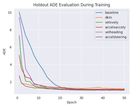
\ The intuition for enforcing kinematic priors comes from the idea that even conditionally independent predicted trajectory waypoints have inherent relationships with each other depending on the state of the agent, even if the neural network does not model it. By propagating these relationships across the time horizon, we focus optimization of the network in the space of kinematically feasible trajectories. We consider four different formulations: 1) with velocity components vx and vy, 2) with acceleration components ax and ay, 3) with speed s = ∥v∥ and heading θ, and finally, 4) with acceleration a (second order of speed) and steering angle δ.
\
- Formulation 1: Velocity Components: The velocity component formulation is the simplest kinematic formulation, where the GMMs predict the distribution of velocity components vx and vy for each timestep t.
\ \ 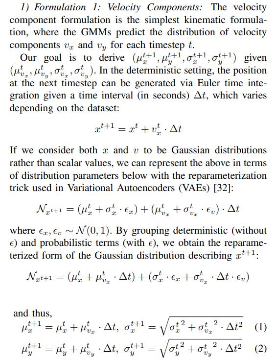
\ \ Also, for the first prediction timestep, we consider the starting trajectory position to represent a distribution with standard deviation equal to zero.
\ This Gaussian form is also intuitive as the sum of two Gaussian random variables is also Gaussian. Since this formulation is not dependent on any term outside of timestep t, distributions for all T timesteps can be computed with vectorized cumulative sum operations. We derive the same distributions in the following sections in a similar fashion with different kinematic parameterizations.
\ \ 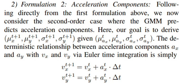
\ \ \ 
\ \ Following similar steps to Formulation 1, we obtain the parameterized distributions of vx and vy:
\ \ 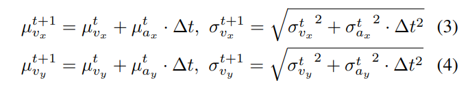
\ \ When computed for all timesteps, we now have T total distributions representing vx and vy, which then degenerates to Formulation 1 in Equation 1.
\ \ 
\ \ When representing this formulation in terms of Gaussian parameters, we point out that the functions cos(·) and sin(·) applied on Gaussian random variables do not produce Gaussians:
\ \ 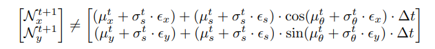
\ \ To amend this, we instead replace cos(·) and sin(·) with linear approximations T(·) evaluated at µθ.
\ \ 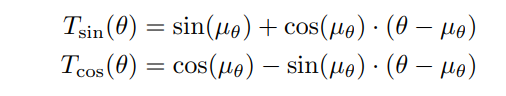
\ \ We now derive the formulation of the distribution of positions with the linear approximations instead:
\ \ 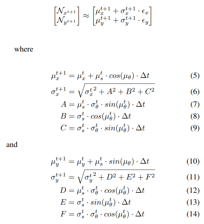
\ \ The full expansion of these terms is described in Section VII-A of the appendix, which can be found on our project page under the title.
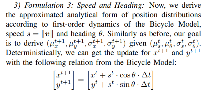
\ 4) Formulation 4: Acceleration and Steering: Lastly, we derive a second-order kinematic formulation based on the bicycle model: steering δ and acceleration a. This formulation is the second-order version of the velocity-heading formulation. Here, we assume acceleration a to be scalar and directionless, in contrast to Formulation 2, where we consider acceleration to be a vector with lateral and longitudinal components. Similarly to Formulation 2, we also use the linear approximation of tan(·) in order to derive approximated position distributions.
\ Following the Bicycle Model, the update for speed and heading at each timestep is:
\ \ 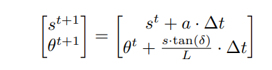
\ \ Where L is the length of the agent. When we represent this process probabilistically as random Gaussian variables, we solve for the distributions of first-order variables, speed (s) and heading (θ):
\ \ 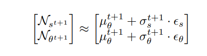
\ \ where
\ \ 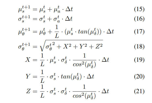
\ \ With the computed distributions of speed and heading, we can then use the analytical definitions from Formulation 3, in Equation 5, to derive the distribution of positions in terms of x and y.
\
C. Error Bound of Linear Approximation.
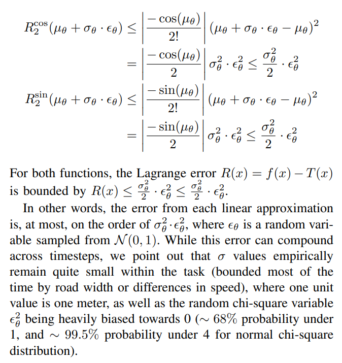
The linear approximations used to derive the variance in predicted trajectories come with some error relative to the actual variance computed from transformations on predicted Gaussian variables, which may not necessarily be easily computable or known. However, we can bound the error of this linear approximation thanks to the alternating property of the sine and cosine Taylor expansions.
\ We analytically derive the error bound for the linear approximation for f(x) = cos(x) and f(x) = sin(x) functions at µθ. Since the Taylor series expansion of both functions are alternating, the error is bounded by the term representing the second order derivative:
\ \ 
\ \ \ ![TABLE I: Performance comparison for vehicles on each kinematic formulation versus SOTA baseline [7] and DKM [1] on Waymo Motion Dataset, Marginal Trajectory Prediction. In our experiments, we downscale the backbone model size from 65M parameters to 2M parameters. From the results, we find that Formulation 3 (speed and heading) provides the greatest and most consistent boost in performance across most metrics over the baseline that does not include kinematic priors.](https://cdn.hackernoon.com/images/fWZa4tUiBGemnqQfBGgCPf9594N2-q1d33l5.png)
\
:::info Authors:
(1) Laura Zheng, Department of Computer Science, University of Maryland at College Park, MD, U.S.A (lyzheng@umd.edu);
(2) Sanghyun Son, Department of Computer Science, University of Maryland at College Park, MD, U.S.A (shh1295@umd.edu);
(3) Jing Liang, Department of Computer Science, University of Maryland at College Park, MD, U.S.A (jingl@umd.edu);
(4) Xijun Wang, Department of Computer Science, University of Maryland at College Park, MD, U.S.A (xijun@umd.edu);
(5) Brian Clipp, Kitware (brian.clipp@kitware.com);
(6) Ming C. Lin, Department of Computer Science, University of Maryland at College Park, MD, U.S.A (lin@umd.edu).
:::
:::info This paper is available on arxiv under ATTRIBUTION-NONCOMMERCIAL-NODERIVS 4.0 INTERNATIONAL license.
:::
\


You May Also Like

How an ideological fracture embroiled Trump DOJ’s push to prosecute enemies

Trump's civil rights chief attended wedding of 'Stop the Steal' organizer: report