The Soup Kitchen Bound: ReLU Inequalities at the Core of Availability vs. Throughput
Table of Links
Abstract and 1. Introduction
-
The Soup Kitchen Problem
2.1 Model and 2.2 Limits of Throughput and Availability
2.3 Analysis of Throughput and Availability
-
Multi-Unit Posted-Price Mechanisms
3.1 Model
3.2 Results
-
Transaction fee mechanism design
-
Conclusions and future work, and References
\ A. Proofs for Section 2 (The Soup Kitchen Problem)
B. Proofs for Section 3 (Multi-Unit Posted-Price Mechanisms)
\
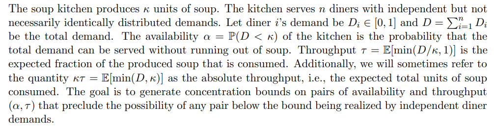
2. The Soup Kitchen Problem
2.1 Model
\
2.2 Limits of Throughput and Availability
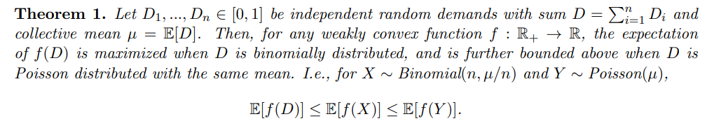
The following high-level sequence of results culminates in our main theorem.
\ 
\ 
\ 
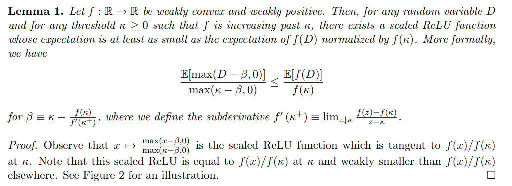
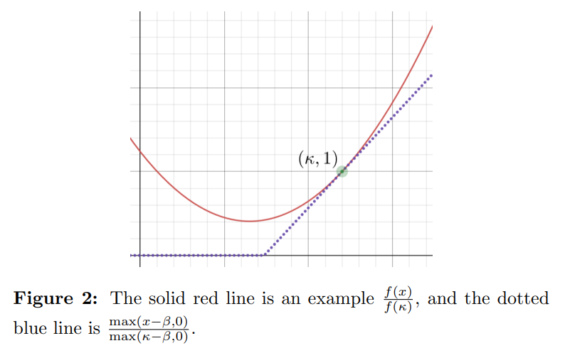
\ Some functions f in the above theorem will produce stronger bounds, while others will produce weaker bounds. The following lemma can be used to narrow the search space for functions f that produce strong bounds:1
\ 
\ 
\
2.3 Analysis of Throughput and Availability
This section sketches the proofs of Theorem 1, Theorem 2, and Theorem 3. Full proofs can be found in the appendix.
\ One way to conceptualize Theorem 1 is that it demonstrates a set of upper bounds on E[f(D)] that are tight when
\ \ 
\ \ To prove Theorem 1, we first show the following lemma:
\ \ 
\ \ \ 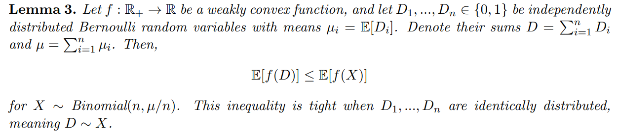
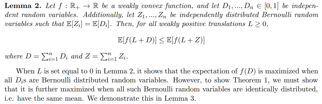
\ \ A proof of Lemma 3 can also be found in other works (Hoeffding, 1956; Arnosti and Ma, 2023), and can be naturally extended to show that E[f(X)] is maximized as the number of demands n → ∞, i.e. as the binomial X approaches a Poisson Y with mean Y] = E[X]. The fact that E[f(X)] ≤ Y)] is used to conclude Theorem 1. Furthermore, observe that E[f(X)] ≤ Y)] additionally implies that the bound in Theorem 3 is weakest when n → ∞.
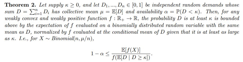
\ The proof of Theorem 2 from Theorem 1 is relatively straightforward. It follows a similar structure to Markov’s inequality on the random variable f(D).
\ Proof of Theorem 2. From the law of total expectation, we have
\ E[f(D)] = E[f(D) 1(D < κ)] + E[f(D) | D ≥ κ]P(D ≥ κ).
\ Since f is weakly positive, E[f(D) 1(D < κ)] ≥ 0. Furthermore, since f is weakly convex, E[f(D) | D ≥ κ] ≥ f(E[D | D ≥ κ]). Thus,
\ f(E[D | D ≥ κ]) P(D ≥ κ) ≤ E[f(D)].
\ Next, from Theorem 1, we have E[f(D)] ≤ E[f(X)]. Therefore,
\ f(E[D | D ≥ κ]) P(D ≥ κ) ≤ E[f(X)].
\ Dividing both sides by f(E[D | D ≥ κ]) ≥ 0, we obtain as desired:
\ \ 
\ \ Observe that the most notable difference between Theorem 2 and Markov’s inequality is that the denominator on the right-hand side is f(E[D | D ≥ κ]), not f(κ).
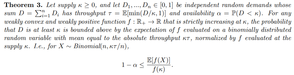
\ Proving Theorem 3 from Theorem 2 is quite involved.
\ Proof sketch of Theorem 3. We select the ReLU mapping f(x) = max(x−β, 0) for a value of β ≤ κ, and obtain
\ \ 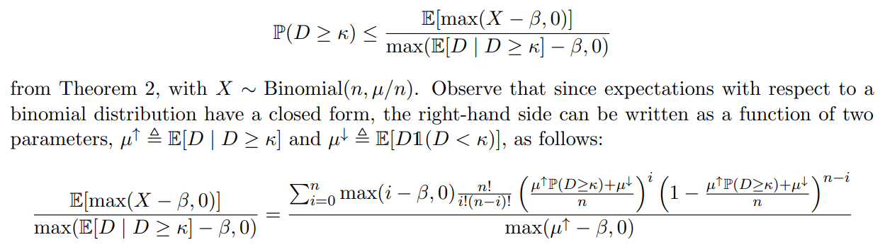
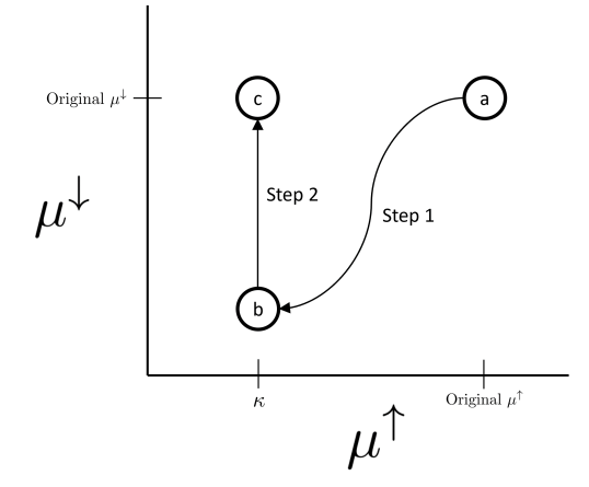
\ \ In the case where β < 0, we show directly that the right-hand side is decreasing in µ ↑, and move µ ↑ → κ. In the more complicated case where β ≥ 0, we adjust the parameters of the right-hand side in two steps:
\
-
Move along a path of pairs (µ↑, µ↓) that keeps the right-hand side constant, and such that the end of the path is the point (κ, t) for some t below the original µ ↓.
\
-
Adjust t upwards to the original µ↓, and show that this only increases the right-hand side.
\ Therefore, the final value of the right-hand side should be at least P(D ≥ κ). See Figure 3 for an illustration.
\ The resulting formula for the right-hand side is equal to the formula for the expectation of a binomial distribution with mean κP(D ≥ κ) + µ ↓ = κτ , divided by the value max(κ − β, 0). A straightforward application of Lemma 1 completes the theorem, showing that this ReLU bound can be weakened to f(X)/f(κ) for X ∼ Binomial(n, κτ /n).
\ Observe that the ReLU function described in Lemma 1 is weakly convex, weakly positive, and is strictly increasing past κ. It thus satisfies all the requirements for making a concentration inequality using Theorem 3, and we can conclude that for any concentration inequality made using Theorem 3, there exists a ReLU function that produces a concentration inequality at least as strong. This means that in order to find the functions f for use with Theorem 3 that produce the strongest concentration inequalities, it suffices to search solely among the class of ReLU functions.
\ \ 
\
:::info Authors:
(1) Aadityan Ganesh, Princeton University (aadityanganesh@princeton.edu);
(2) Jason Hartline, Northwestern University (hartline@northwestern.edu);
(3) Atanu R Sinha, Adobe Research (atr@adobe.com);
(4) Matthew vonAllmen, Northwestern University (matthewvonallmen2026@u.northwestern.edu).
:::
:::info This paper is available on arxiv under CC BY 4.0 DEED license.
:::
\


추천 콘텐츠

Markets price future Middle East de-escalation – Danske Bank

Forex Markets Brace for Impact as Trump’s Critical Deadline Looms