BCD‑SCA Based Optimization for UAV‑CRN: Joint Trajectory, Power, and Scheduling Design
Table of Links
Abstract and I. Introduction
II. System Model
III. Problem Formulation
IV. Proposed Algorithm for Problem P0
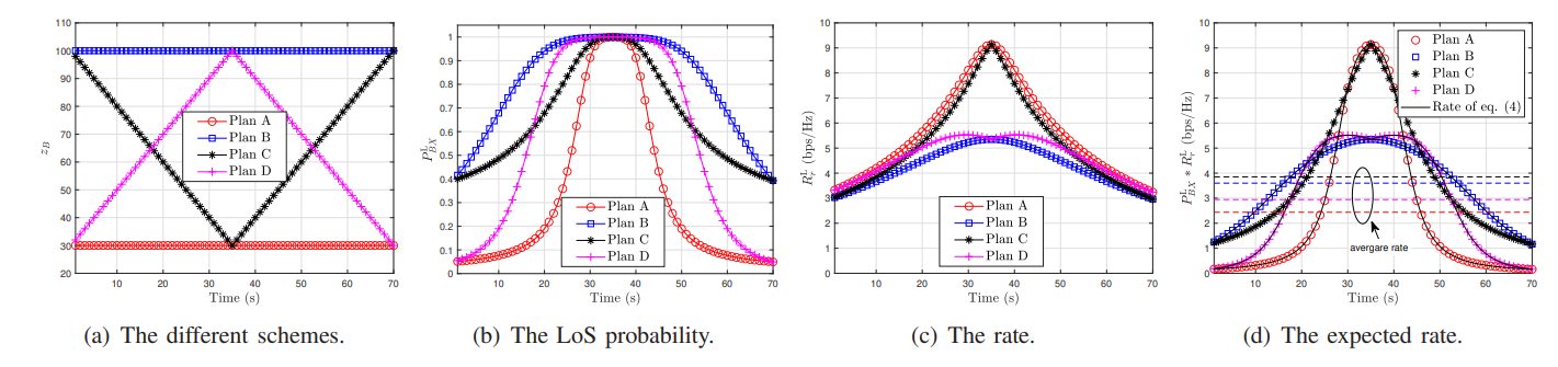
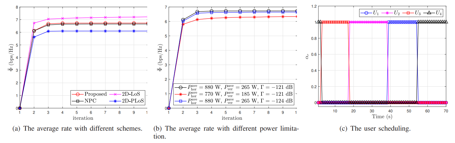
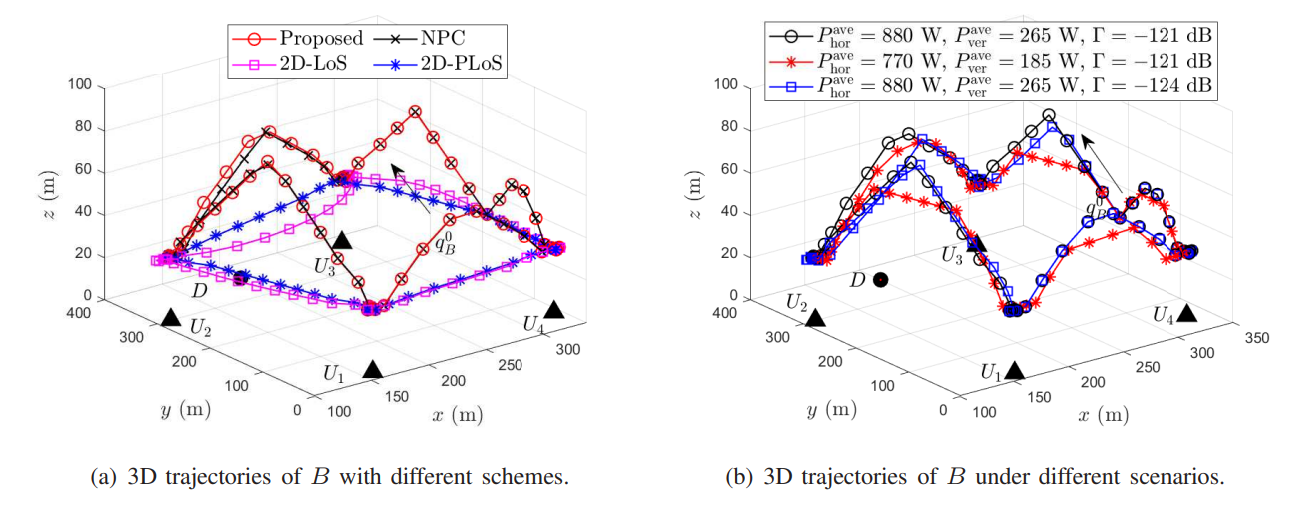
V. Numerical Results
VI. Conclusion
APPENDIX A: PROOF OF LEMMA 1 and References
II. SYSTEM MODEL
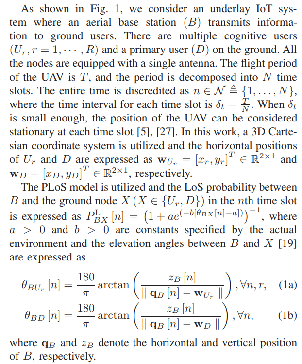
\ The channel coefficient between B and X in the nth time slot is expressed a
\ 
\ 
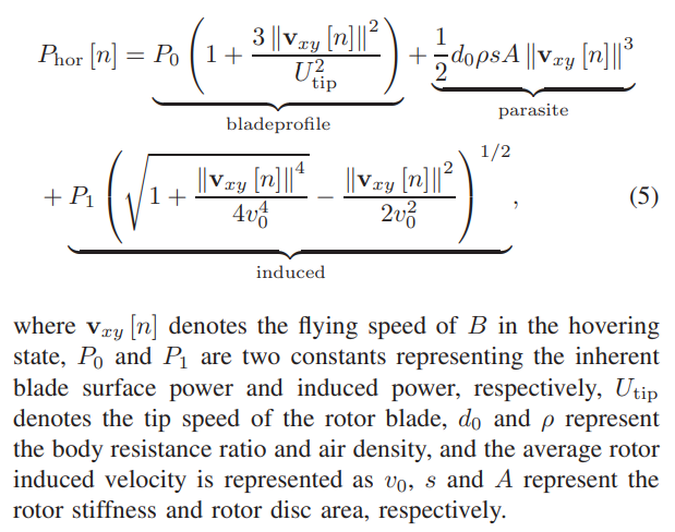
\ The horizontal energy consumption of B is expressed as [14]
\ 
\ The energy consumption of B in the vertical direction is as expressed as [24], [39]
\ 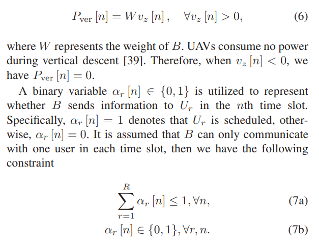
\ 
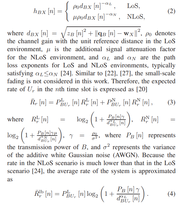
\ The average rate of the considered system is expressed as
\ 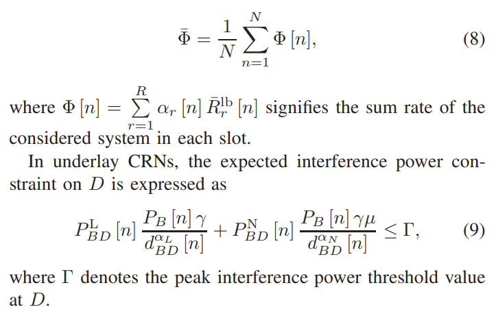
\
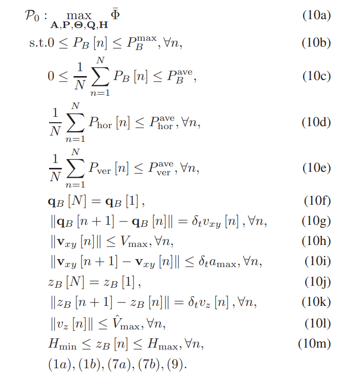
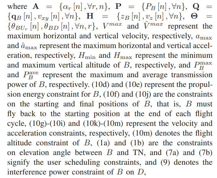
III. PROBLEM FORMULATION
In this work, the average rate of the system is optimized, which is related to user scheduling, the transmission power and 3D trajectory, the horizontal and vertical velocities of B. Then the following optimization problem is formulated
\ \ 
\ \ \ 
\ \ \ 
\
IV. PROPOSED ALGORITHM FOR PROBLEM P0
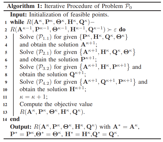
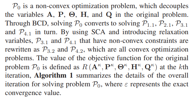
To solve P0, we utilize the BCD technology to decompose the original problem into multiple subproblems. Specifically, for the given other variables, A, P, H, and Q are optimized in each subproblem respectively. In addition, the SCA technology is utilized to transform the non-convex constraints into convex constraints.
\ A. Subproblem 1: Optimizing User Scheduling Variable
\ \ 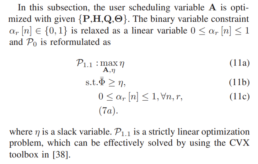
\ \ \ 
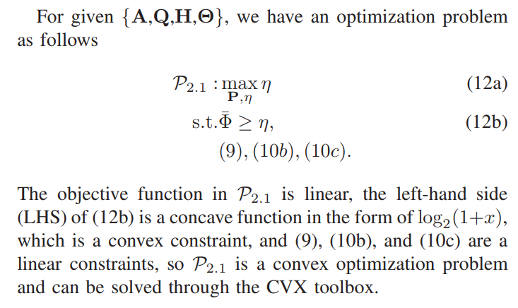
\ \ B. Subproblem 2: Optimizing Transmit Power of B
\ \ 
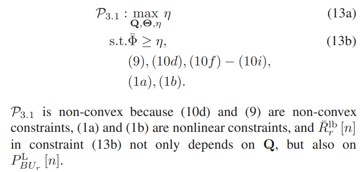
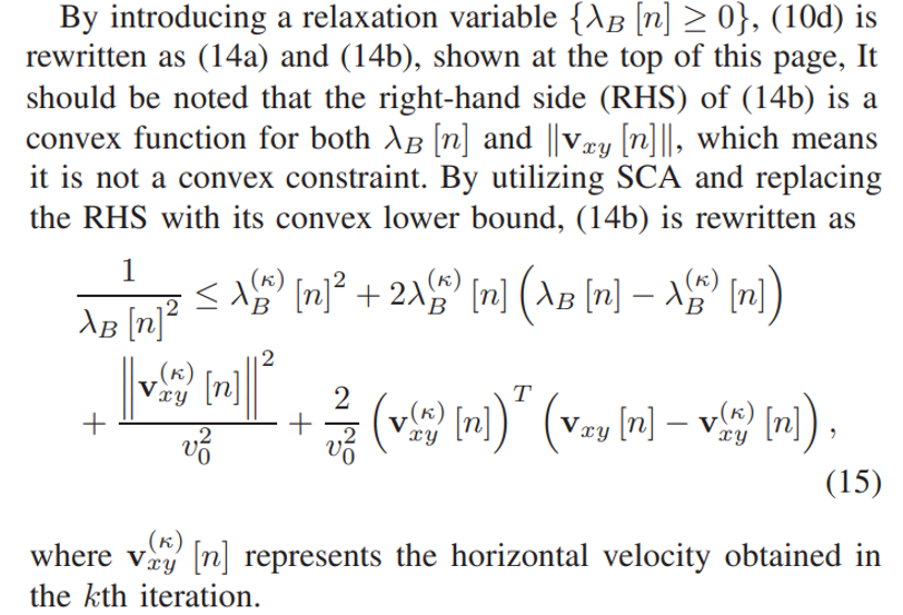
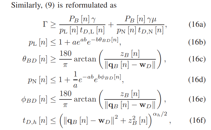
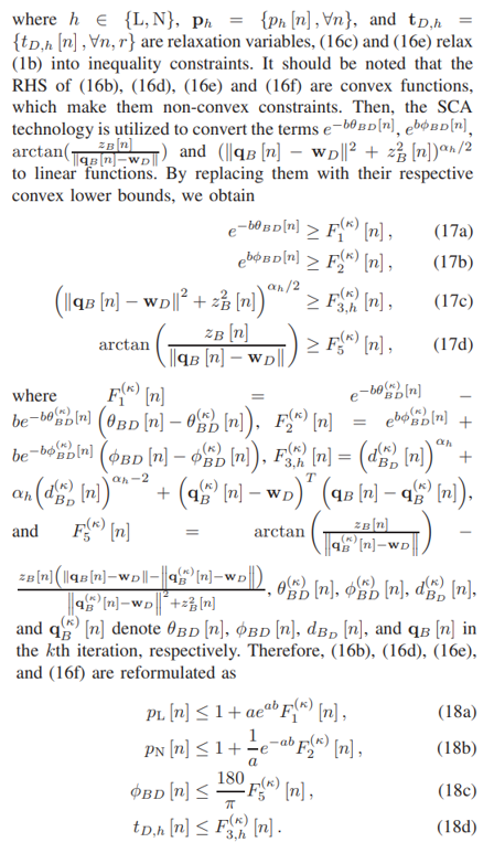
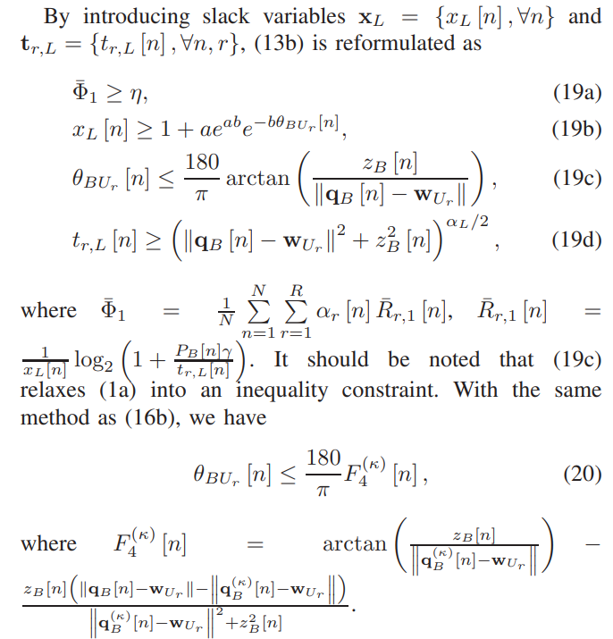
\ \ C. Subproblem 3: Optimizing Horizontal Trajectory and Velocity of B
\ In this subsection, the horizontal trajectory and velocity of B is optimized for provided {A,P,H}. The original optimization problem is rewritten as
\ \ 
\ \ \ 
\ \ \ 
\ \ \ 
\ \ \ 
\ \ To address the non-convexity in (19a), Lemma 1 is introduced.
\ \ 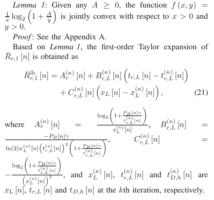
\ \ \ 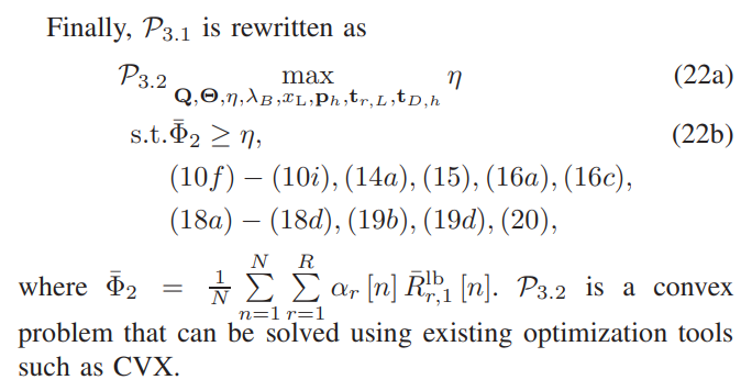
\ \ D. Subproblem 4: Optimizing Horizontal Trajectory and Velocity of B
\ In this subsection, for given {A,P,Q}, the vertical trajectory H of B is optimized. The optimization problem is expressed as
\ \ 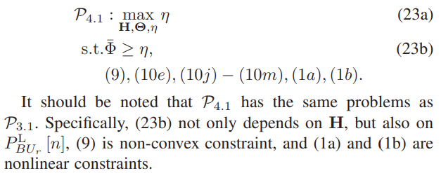
\ \ With the same method as (13b), (23b) is reformulated as (19a)-(19d) and (1a) and (1b) are reformulated as (16c), (16e), and (19c). With the same method in Subproblem 3, (9) in this subsection is reformulated as (16a)-(16f) wherein (16b) and (16d) are reformulated as (18a) and (18b), respectively.
\ \ 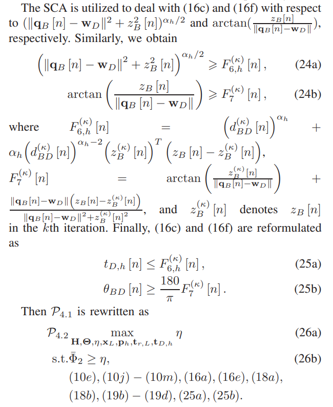
\ \ \ 
\ \ P4.2 is a convex optimization problem that can be solved using existing optimization tools such as CVX.
\ E. Convergence Analysis of Algorithm 1
\ \ 
\ \ The obtained suboptimal solution of the transformed subproblem is also the suboptimal solution of the original nonconvex subproblem, and each subproblem is solved using SCA convex transformation iteration. Finally, all suboptimal solutions of the subproblems that satisfy the threshold ε constitute the suboptimal solution of the original problem. Therefore, our algorithm is to alternately solve the subproblem P1.1, P2.1, P3.2 and P4.2 to obtain the suboptimal solution of the original problem until a solution that satisfies the threshold ε is obtained.
\ It is worth noting that in the classic BCD, to ensure the convergence of the algorithm, it is necessary to accurately solve and update the subproblems of each variable block with optimality in each iteration. But when we solve P3.1 and P4.1 , we can only optimally solve their approximation problem P3.2 and P4.2. Therefore, we cannot directly apply the convergence analysis of the classical BCD, and further proof of the convergence of Algorithm 1 is needed, as shown below.
\ \ 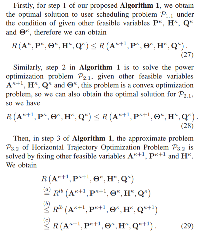
\ \ \ 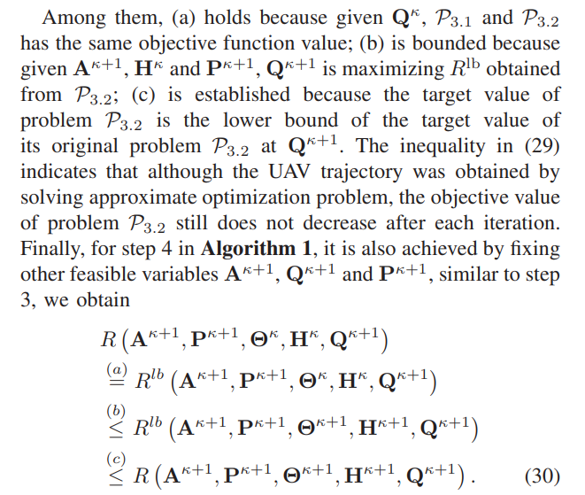
\ \ (30) This is similar to the representation in (29), and from (27) to (30), we obtain
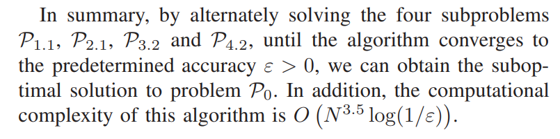
\ 1 . (31) The above analysis indicates that the target value of P0 does not decrease after each iteration of Algorithm 1. Due to the objective value of P0 is a finite upper bound, therefore the proposed Algorithm 1 ensures convergence. The simulation results in the next section indicate that the proposed BCDbased method converges rapidly for the setting we are considering. In addition, since only convex optimization problems need to be solved in each iteration of Algorithm 1, which have polynomial complexity, Algorithm 1 can actually converge
\ \ 
\ \ \ 
\ \ quickly for wireless networks with a moderate number of users.
\ \ 
\
:::info Authors:
(1) Hongjiang Lei, School of Communications and Information Engineering, Chongqing University of Posts and Telecommunications, Chongqing 400065, China (leihj@cqupt.edu.cn);
(2) Xiaqiu Wu, School of Communications and Information Engineering, Chongqing University of Posts and Telecommunications, Chongqing 400065, China (cquptwxq@163.com);
(3) Ki-Hong Park, CEMSE Division, King Abdullah University of Science and Technology (KAUST), Thuwal 23955-6900, Saudi Arabia (kihong.park@kaust.edu.sa);
(4) Gaofeng Pan, School of Cyberspace Science and Technology, Beijing Institute of Technology, Beijing 100081, China (gaofeng.pan.cn@ieee.org).
:::
:::info This paper is available on arxiv under CC BY 4.0 DEED license.
:::
\


추천 콘텐츠

Monetary Policy Stays Steady As Geopolitical Storm Clouds Gather

Schwab Trading Activity Index™: STAX Score Sees Steepest Monthly Drop Since May 2025