A Practical Guide to G-LSM: Improving High-Dimensional Option Pricing with Minimal Overhead
Table of Links
Abstract and 1. Introduction
- Bermudan option pricing and hedging
- Sparse Hermite polynomial expansion and gradient
- Algorithm and complexity
- Convergence analysis
- Numerical examples
- Conclusions and outlook, Acknowledgments, and References
\ 
\ 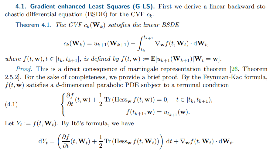
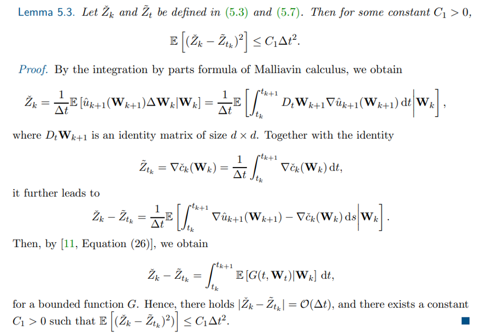
\ In view of (4.1), the drift term vanishes. After taking the stochastic integral and using the terminal condition in (4.1), we obtain the desired assertion.
\ \ 
\ 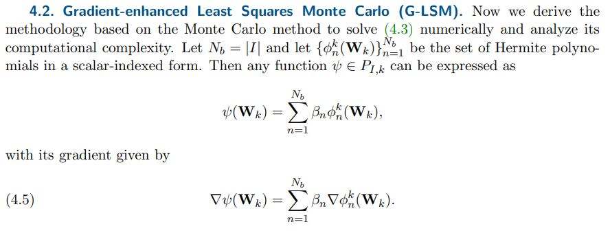
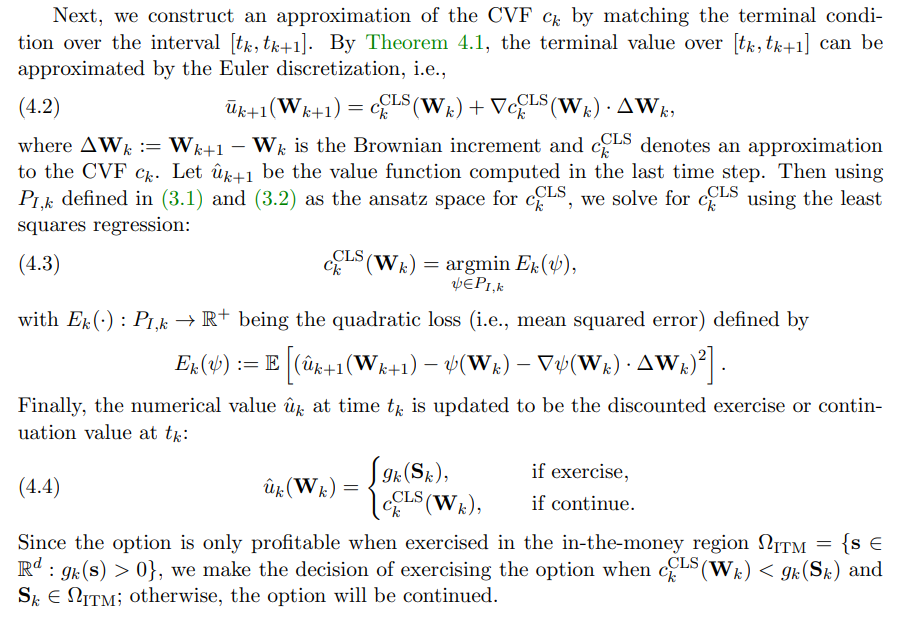
\ In practice, the continuous least squares problem (4.3) is solved by minimizing its Monte Carlo approximation:
\ 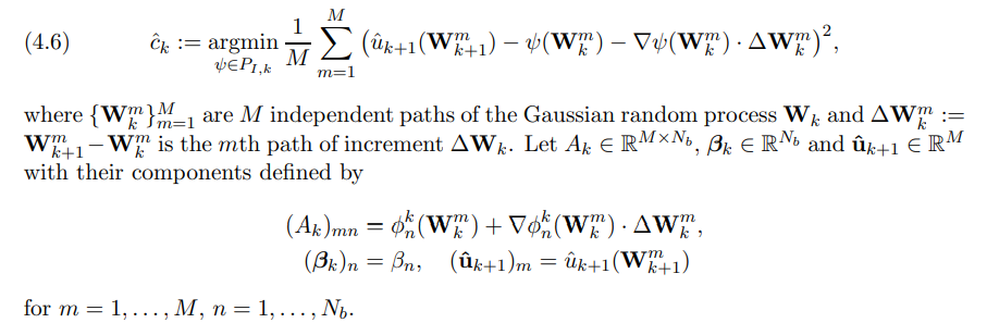
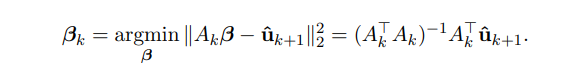
\ Then finding the optimal polynomial in (4.6) amounts to solving the classical least squares problem
\ 
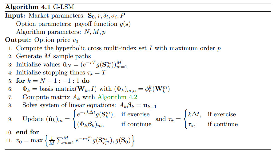
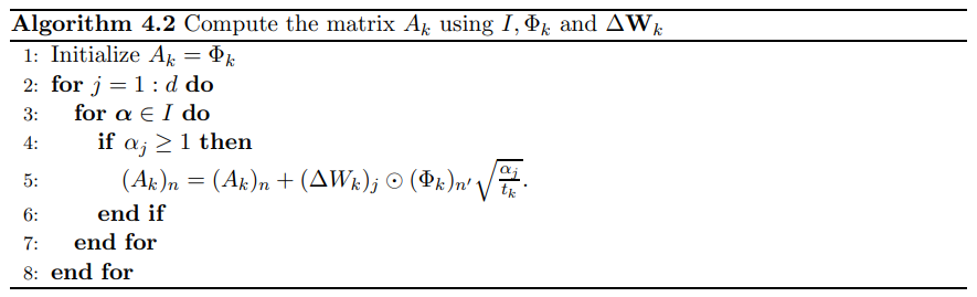
\ The proposed algorithm is summarized in Algorithm 4.1.
\ 
\ 
\ 
\ 
\ 
\ 
\ 
\ 5. Convergence analysis. Now we analyze the convergence of Algorithm 4.1. We assume the Lipschitz continuity of the discounted payoff function gk(·).
\ \ 
\ \ \ 
\ \ \ 
\ \ \ 
\ \ \ 
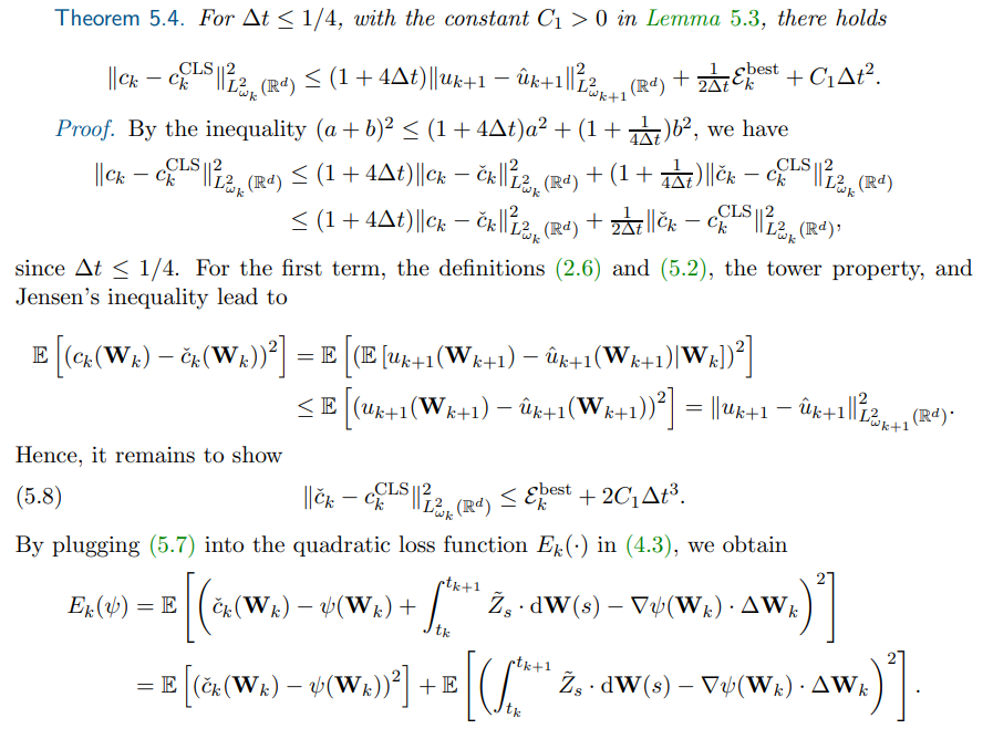
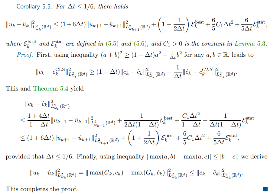
\ \ Next, we provide an error estimate of solving the continuous least squares problem (4.3) in terms of the error of the previous value function, the best approximation error in the sparse Hermite polynomial ansatz space (5.5) and the time step size ∆t. The proof is inspired by the foundational work [12].
\ \ 
\ \ \ 
\ \ \ 
\ \ \ 
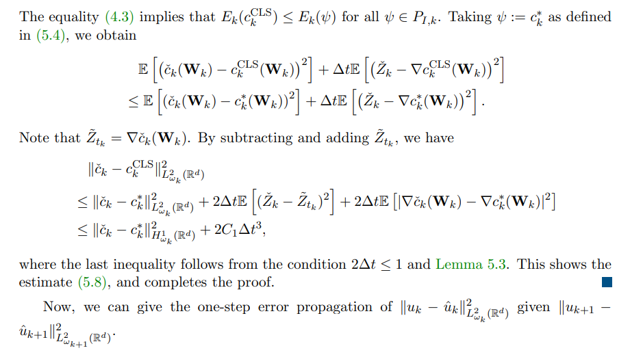
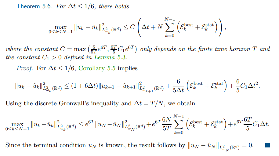
\ \ 5.2. Global error estimation. Finally, we prove a global error estimate.
\ \ 
\ \ \ 
\ \ \ 
\ \ \ 
\ \ \ 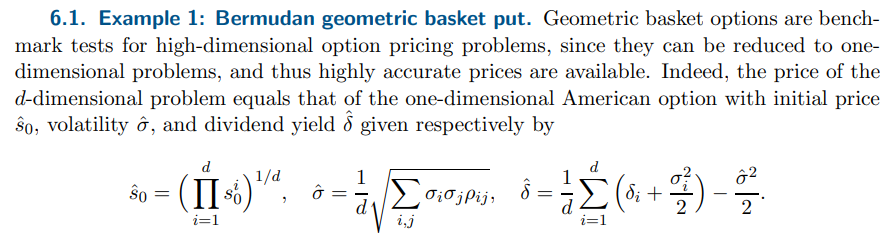
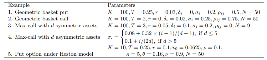
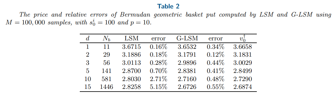
\ \ We consider the example of Bermudan geometric basket put from [13, 25]. The exact prices are computed by solving the reduced one-dimensional problem via a quadrature and interpolation-based method [25] for Bermudan options. We present in Table 2 the computed option prices and their relative errors using G-LSM and LSM, with the same ansatz space for the CVF. The results show that G-LSM achieves higher accuracy than LSM in high-dimensions: G-LSM has a relative error 0.55% for d = 15, which is almost ten times smaller than that by LSM. That is, by incorporating the gradient information, the accuracy of LSM can be substantially improved.
\ \ 
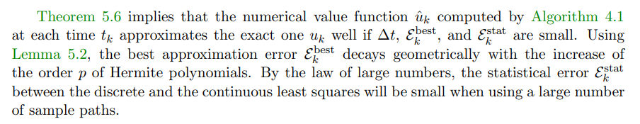
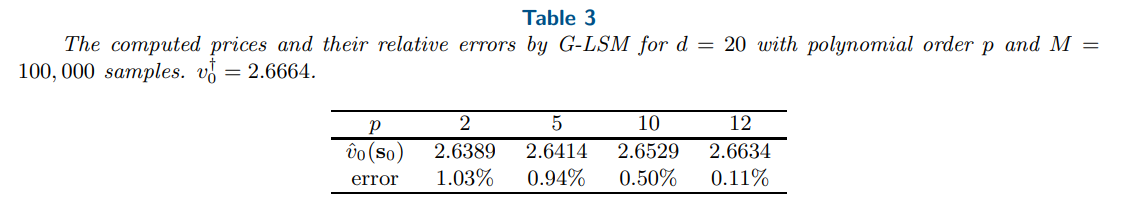
\ \ Table 3 gives the computed option prices and their relative errors by G-LSM with different maximum polynomial orders p for the 20-dimensional geometric basket put. The relative error decays steadily as the order p of Hermite polynomials increases, which agrees with Theorem 5.6.
\ \ 
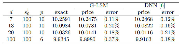
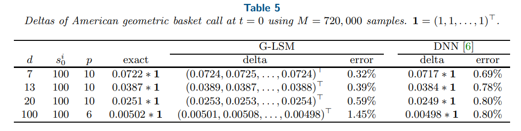
\ \ 6.2. Example 2: American geometric basket call. Now we consider the example of American geometric basket call option from [21, 6] to demonstrate that the proposed G-LSM can achieve the same level of accuracy as the DNN-based method [6], and take M = 720, 000 samples as in [6]. The prices and deltas are given in Table 4 and Table 5, respectively, where the results of [6] are the average of 9 independent runs. From Table 4, both methods have similar accuracy for the price. From Table 5, the relative error of delta using G-LSM and DNN varies slightly with the dimension d. This is probably because the DNN-based method computes the delta via a sample average, while G-LSM uses the derivatives of the value function directly. The relative error of the delta computed by G-LSM increases slightly for larger dimensions, possibly due to the small magnitude of the exact delta values.
\ \ 
\ \ \ 
\ \ \ 
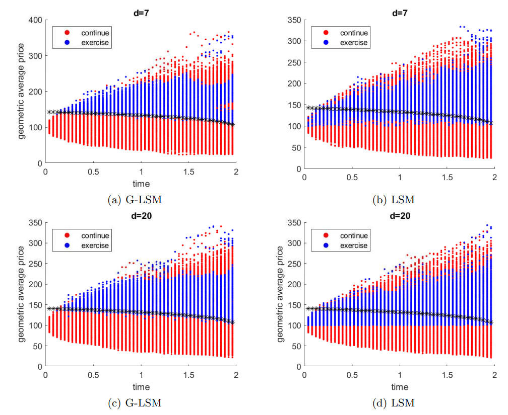
\ \ Next, Figure 2 shows the classification results of continued and exercised data using GLSM and LSM with the number of simulated paths M = 100, 000 in d = 7 or 20. Compared with the exact exercise boundary, G-LSM achieves better accuracy in determining the exercise boundary than LSM despite of using the same ansatz and number of paths. Thus, even with the right ansatz space, LSM might fail the task of finding exercise boundary in high dimensions using only a limited number of samples. Compared with [6, Figure 5] and [18, Figure 6], Figure 2 demonstrates that G-LSM can detect accurate exercise boundary with fewer number of paths than the DNN-based method.
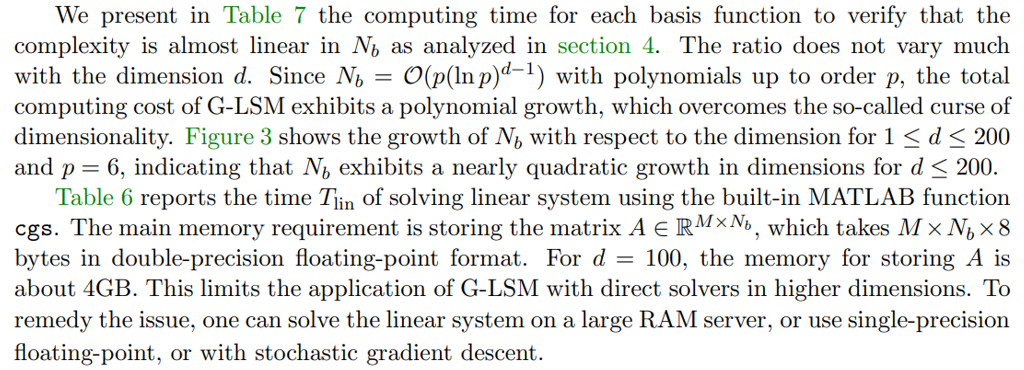
\ 6.3. Example 3: Bermudan max-call with symmetric assets. To benchmark G-LSM on high-dimensional problems without exact solutions and to validate the complexity analysis in section 4, we test Bermudan max-call option and report the computing time. The computing time is calculated as follows. For a fixed time step, Tbas is the time for generating basis matrix Φ, Tmat is the time for assembling matrix A, Tlin is the time for solving linear system, and Tup is the time for updating values. The overall computing time is Ttot ≈ (N − 1)(Tbas + Tmat + Tlin + Tup).
\ Table 6 presents the prices and computing time (in seconds) for Bermudan max-call options with d symmetric assets. The reference 95% confidence interval (CI) is taken from [3]. The reference CI is computed with more than 3000 training steps and a batch of 8192 paths in each step, which in total utilizes more than 107 paths. The last five columns of the table report the computing time for the step 6, 7, 8, 9 in Algorithm 4.1, and the total time, respectively. All the computation for this example was performed on an Intel Core i9-10900 CPU 2.8 GHz desktop with 64GB DDR4 memory using MATLAB R2023b. It is observed that the prices computed by G-LSM fall into or stay very close to the reference 95% CI, confirming the high accuracy of G-LSM. Furthermore, the time for generating basis matrix, Tbas, dominates the
\ \ 
\ \ overall computing time. Hence, the cost mainly arises from evaluating Hermite polynomials on sampling paths, which is also required by LSM. In comparison with LSM , Tmat is the extra cost to incorporate the gradient information and takes only a small fraction of the total time. Therefore, G-LSM has nearly identical cost with LSM.
\ \ 
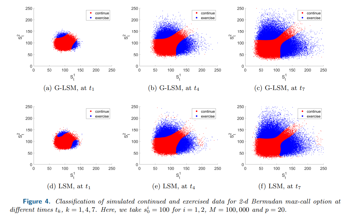
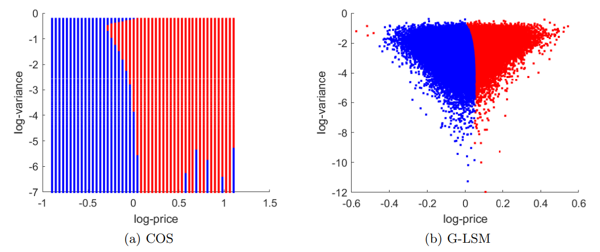
\ \ Figure 4 shows the classification of continued and exercised sample points computed by G-LSM and LSM in the example of two-dimensional max-call. G-LSM yields a smoother exercise boundary than LSM. Compared with the exercise boundary computed in literature [19, Figure 3], G-LSM exhibits higher accuracy, albeit that the same ansatz space for the CVF is employed.
\ \ 
\ \ \ 
\ \ \ 
\ \ \ 
\ \ \ 
\ \ \ 
\ \ \ 
\ \ \ 
\ 7. Conclusions and outlook. In this work, we have proposed a novel gradient-enhanced least squares Monte Carlo (G-LSM) method that employs sparse Hermite polynomials as the ansatz space to price and hedge American options. The method enjoys low complexity for the gradient evaluation, ease of implementation and high accuracy for high-dimensional problems. We analyzed rigorously the convergence of G-LSM based on the BSDE technique, stochastic and Malliavin calculus. Extensive benchmark tests clearly show that it outperforms least squares Monte Carlo (LSM) in high dimensions with almost the same cost and it can also achieve competitive accuracy relative to the deep neural networks-based methods.
\ \ 
\ \ Acknowledgments. The authors acknowledge the support of research computing facilities offered by Information Technology Services, the University of Hong Kong.
REFERENCES
[1] B. Adcock, S. Brugiapaglia, and C. G. Webster, Sparse Polynomial Approximation of HighDimensional Functions, SIAM, Philadelphia, PA, 2022.
\ [2] C. Bayer, M. Eigel, L. Sallandt, and P. Trunschke, Pricing high-dimensional Bermudan options with hierarchical tensor formats, SIAM Journal on Financial Mathematics, 14 (2023), pp. 383–406.
\ [3] S. Becker, P. Cheridito, and A. Jentzen, Deep optimal stopping, The Journal of Machine Learning Research, 20 (2019), pp. 2712–2736.
\ [4] S. Becker, P. Cheridito, and A. Jentzen, Pricing and hedging American-style options with deep learning, Journal of Risk and Financial Management, 13 (2020), p. 158.
\ [5] B. Bouchard and X. Warin, Monte-Carlo valuation of American options: facts and new algorithms to improve existing methods, in Numerical Methods in Finance: Bordeaux, June 2010, Springer, Berlin, 2012, pp. 215–255.
\ [6] Y. Chen and J. W. Wan, Deep neural network framework based on backward stochastic differential equations for pricing and hedging American options in high dimensions, Quantitative Finance, 21 (2021), pp. 45–67.
\ [7] W. E, J. Han, and A. Jentzen, Deep learning-based numerical methods for high-dimensional parabolic partial differential equations and backward stochastic differential equations, Communications in Mathematics and Statistics, 5 (2017), pp. 349–380.
\ [8] N. El Karoui, C. Kapoudjian, E. Pardoux, S. Peng, and M.-C. Quenez, Reflected solutions of backward SDE’s, and related obstacle problems for PDE’s, The Annals of Probability, 25 (1997), pp. 702–737.
\ [9] F. Fang and C. W. Oosterlee, A Fourier-based valuation method for Bermudan and barrier options under Heston’s model, SIAM Journal on Financial Mathematics, 2 (2011), pp. 439–463.
\ [10] C. Gao, S. Gao, R. Hu, and Z. Zhu, Convergence of the backward deep bsde method with applications to optimal stopping problems, SIAM Journal on Financial Mathematics, 14 (2023), pp. 1290–1303.
\ [11] E. Gobet and C. Labart, Error expansion for the discretization of backward stochastic differential equations, Stochastic Processes and their Applications, 117 (2007), pp. 803–829.
\ [12] C. Hur´e, H. Pham, and X. Warin, Deep backward schemes for high-dimensional nonlinear PDEs, Mathematics of Computation, 89 (2020), pp. 1547–1579.
\ [13] P. Kovalov, V. Linetsky, and M. Marcozzi, Pricing multi-asset American options: A finite element method-of-lines with smooth penalty, Journal of Scientific Computing, 33 (2007), pp. 209–237.
\ [14] B. Lapeyre and J. Lelong, Neural network regression for Bermudan option pricing, Monte Carlo Methods and Applications, 27 (2021), pp. 227–247.
\ [15] F. Longstaff and E. Schwartz, Valuing American options by simulation: a simple least-squares approach, The Review of Financial Studies, 14 (2001), pp. 113–147.
\ [16] M. Ludkovski, Kriging metamodels and experimental design for Bermudan option pricing, Journal of Computational Finance, 22 (2018), pp. 37–77.
\ [17] X. Luo, Error analysis of the Wiener–Askey polynomial chaos with hyperbolic cross approximation and its application to differential equations with random input, Journal of Computational and Applied Mathematics, 335 (2018), pp. 242–269.
\ [18] A. S. Na and J. W. L. Wan, Efficient pricing and hedging of high-dimensional American options using deep recurrent networks, Quantitative Finance, 23 (2023), pp. 631–651.
\ [19] A. M. Reppen, H. M. Soner, and V. Tissot-Daguette, Deep stochastic optimization in finance, Digital Finance, 5 (2023), pp. 91–111.
\ [20] R. Seydel and R. Seydel, Tools for computational finance, vol. 3, Springer, 2006.
\ [21] J. Sirignano and K. Spiliopoulos, DGM: A deep learning algorithm for solving partial differential equations, Journal of Computational Physics, 375 (2018), pp. 1339–1364.
\ [22] J. Tsitsiklis and B. Van Roy, Regression methods for pricing complex American-style options, IEEE Transactions on Neural Networks, 12 (2001), pp. 694–703.
\ [23] H. Wang, H. Chen, A. Sudjianto, R. Liu, and Q. Shen, Deep learning-based BSDE solver for LIBOR market model with application to Bermudan swaption pricing and hedging, arXiv preprint arXiv:1807.06622, (2018).
\ [24] Y. Wang and R. Caflisch, Pricing and hedging American-style options: a simple simulation-based approach, The Journal of Computational Finance, 13 (2009), pp. 95–125.
\ [25] J. Yang and G. Li, On sparse grid interpolation for American option pricing with multiple underlying assets, arXiv preprint arXiv:2309.08287, (2023).
\ [26] J. Zhang, Backward stochastic differential equations, Springer, 2017.
\
:::info Authors:
(1) Jiefei Yang, †Department of Mathematics, University of Hong Kong, Pokfulam, Hong Kong (jiefeiy@connect.hku.hk);
(2) Guanglian Li, Department of Mathematics, University of Hong Kong, Pokfulam, Hong Kong (lotusli@maths.hku.hk).
:::
:::info This paper is available on arxiv under CC by 4.0 Deed (Attribution 4.0 International) license.
:::
\


You May Also Like

Standard Chartered (STAN.L) Stock; Rises as $12M A*STAR AI Lab Boosts Innovation

Vanguard Increases Strategy Stake to $255M as MSTR Adds $2.54 Billion Bitcoin