Why “Immediacy Bias” Might Be the Secret to Faster, Smarter Blockchain Transactions

Table of Links

Abstract and 1. Introduction

1.1 Our Approach

1.2 Our Results & Roadmap

1.3 Related Work

1. Model and Warmup and 2.1 Blockchain Model

   2.2 The Miner

   2.3 Game Model

   2.4 Warm Up: The Greedy Allocation Function

2. The Deterministic Case and 3.1 Deterministic Upper Bound

   3.2 The Immediacy-Biased Class Of Allocation Function

3. The Randomized Case

4. Discussion and References

• A. Missing Proofs for Sections 2, 3
• B. Missing Proofs for Section 4
• C. Glossary

3 The Deterministic Case

In this section, we focus on the discount model with miner ratio α ̸= 0 and some discount rate λ. Missing proofs are given in Appendix A.

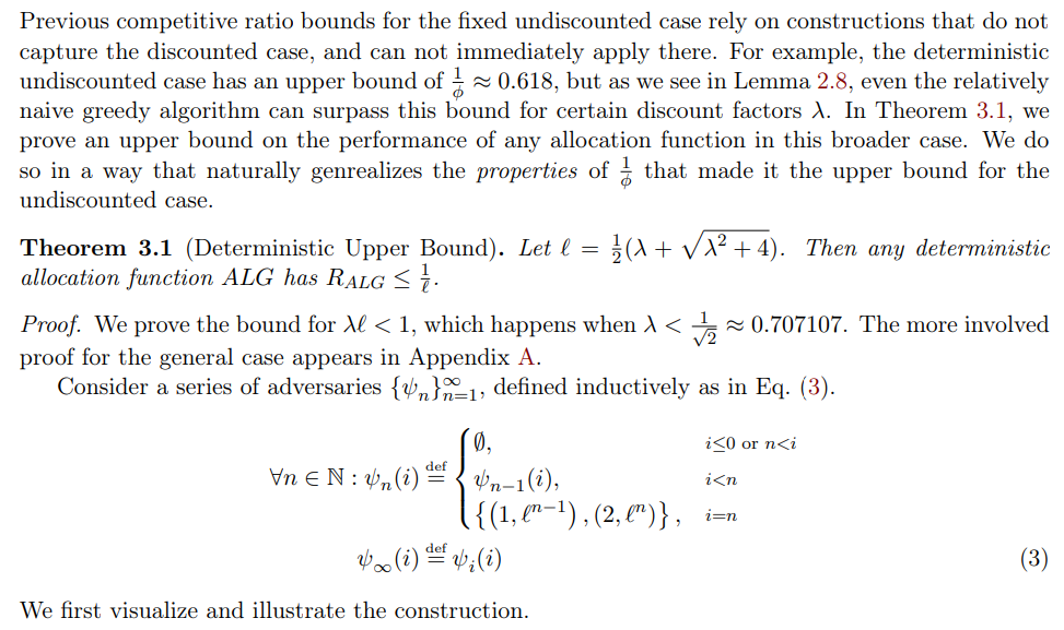
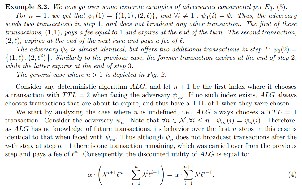
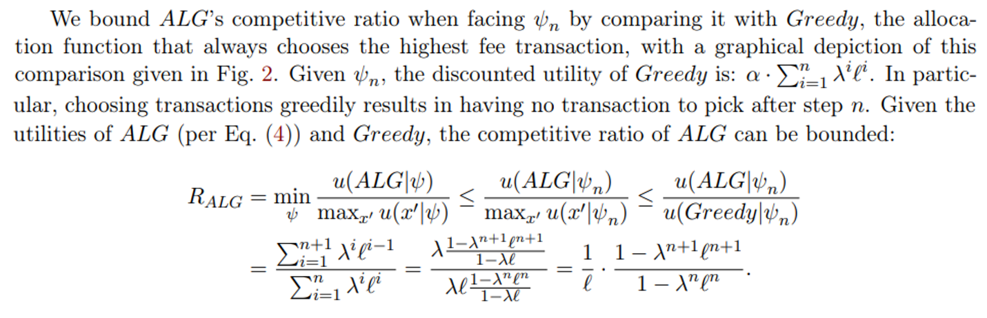
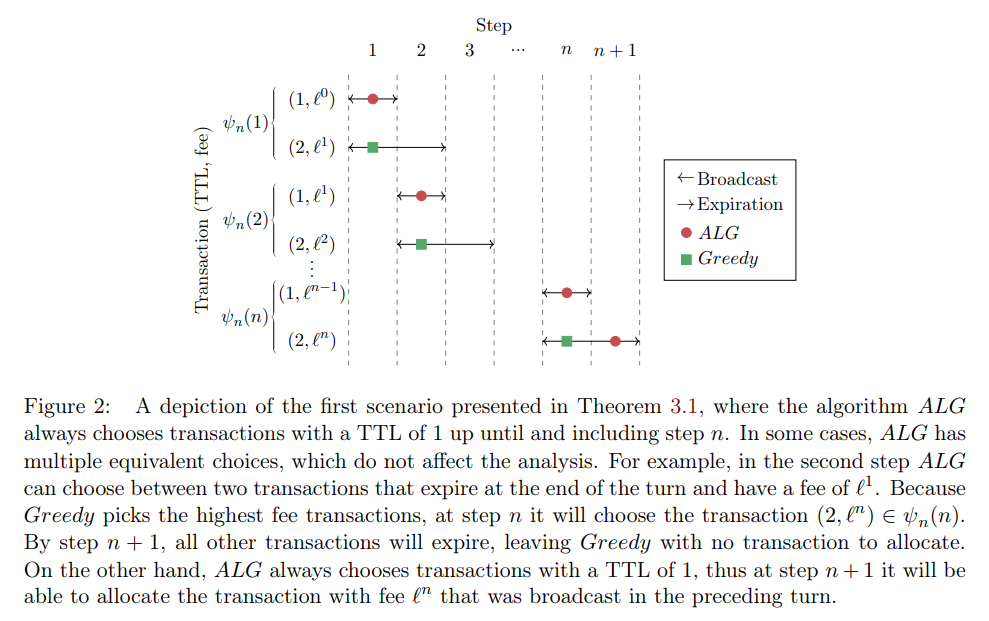
3.1 Deterministic Upper Bound

\

\

\

\

\

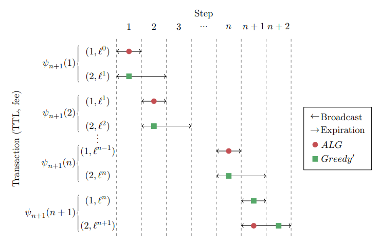
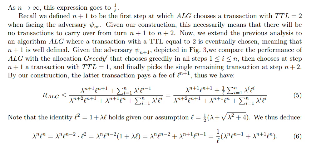
\ By combining Eqs. (5) and (6), the proof is concluded:

\

\

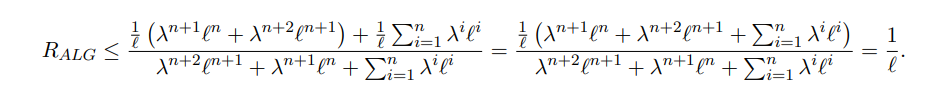
3.2 The Immediacy-Biased Class Of Allocation Function

We proceed by introducing the immediacy-biased ratio class of allocation functions, and identify a regime of discount rates λ which we call the “semi-myopic” regime where it achieves the optimal deterministic competitive ratio. Given a parameter ℓ ∈ R, we denote the corresponding instance of this class as ρℓ and define it in the following manner

\ Definition 3.3 (The ℓ-immediacy-biased ratio allocation function ρℓ). For a set S, let

\ \

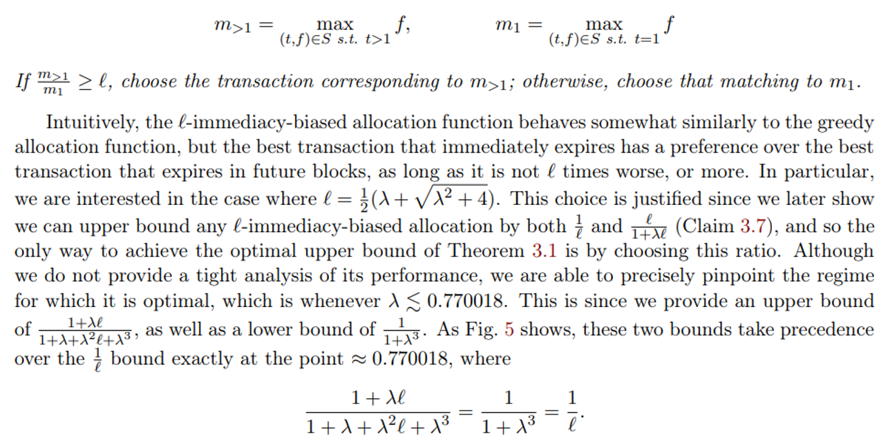
\ \ Before providing the lower and upper bound analysis, we comment on how our algorithm stands in comparison with another algorithm, MG [LSS05]. While the ℓ-immediacy-biased considers only the highest T T L = 1 transaction as a possible candidate to be scheduled instead of the highest-fee transaction, MG considers any earliest-deadline transaction. I.e., the algorithms differ in their behavior when no T T L = 1 transactions are available. However, in terms of competitive analysis, ℓ-immediacy-biased dominates ℓ-MG. That is because at any case that the ℓ-immediacy-biased allocation chooses a T T L = 1 transaction, ℓ-MG would do the same. But any case that ℓ-immediacy-biased allocation chooses the highest-fee transaction; we can force ℓ-MG to do the same by adding a (1, ϵ) with small enough ϵ to the adversary’s schedule at that step. Therefore, we can force ℓ-MG to make the same choices as ℓ-immediacy-biased allocation, without changing the optimal allocation performance.

\ We bound the allocation function’s competitive ratio from below in Lemma 3.4.

\ \

\ \ \

\ \

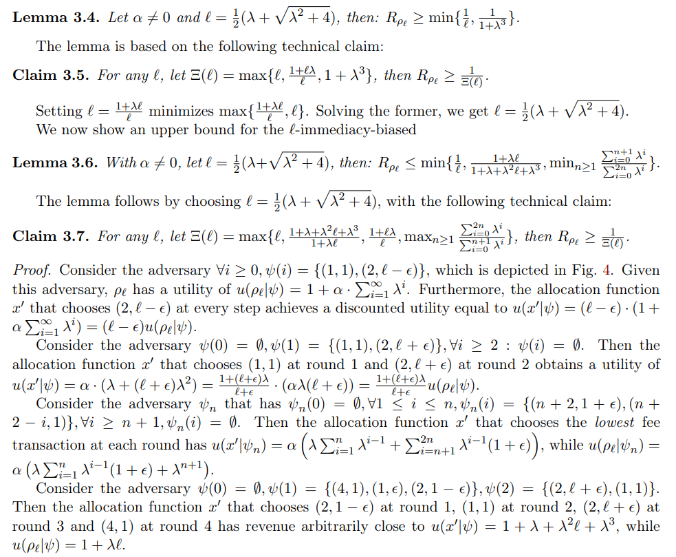
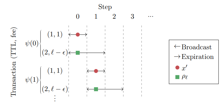
4 The Randomized Case

Next, Theorem 4.1 obtains an upper bound on the competitive ratio of any allocation function.

4.1 Randomized Upper Bound

Theorem 4.1. Given α ̸= 0, for any (possibly randomized) allocation function ALG:

\ \

\ \ Similarly to the deterministic upper bound, the proof uses a recursive construction of adversaries where the transaction fees grow exponentially. The main technical choice is how to decide the base of the exponent. We guess it by the following equation:

\ \

\

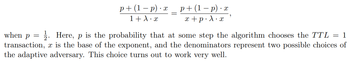
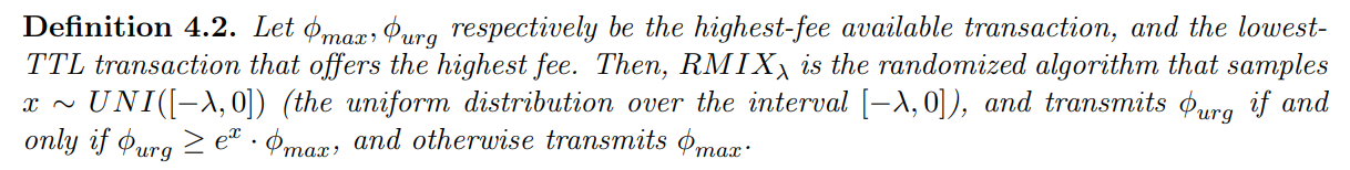
4.2 The RMIXλ Randomized Allocation Function

Next, we show that the best-known randomized allocation function known for the undiscounted case [CCFJST06], extends to the more general discount model.

\ \

\ \ \

\ \ \

\ \ Notably, in the semi-myopic range that we identify in Section 3.2, our simple deterministic allocation achieves very similar performance to the above randomized allocation function.

\ Our competitive ratio results are summarized in Fig. 5.

\

:::info Authors:

(1) Yotam Gafni, Weizmann Institute (yotam.gafni@gmail.com);

(2) Aviv Yaish, The Hebrew University, Jerusalem (aviv.yaish@mail.huji.ac.il).

:::

:::info This paper is available on arxiv under CC BY 4.0 DEED license.

:::

\