Twin‑Tower Neural Architecture for Δ‑Estimation in Differential Financial Models

Table of Links

Abstract

1. Keywords and 2. Introduction

2. Set up

3. From Classical Results into Differential Machine Learning

   4.1 Risk Neutral Valuation Approach

   4.2 Differential Machine learning: building the loss function

4. Example: Digital Options

5. Choice of Basis

   6.1 Limitations of the Fixed-basis

   6.2 Parametric Basis: Neural Networks

6. Simulation-European Call Option

   7.1 Black-Scholes

   7.2 Hedging Experiment

   7.3 Least Squares Monte Carlo Algorithm

   7.4 Differential Machine Learning Algorithm

7. Numerical Results

8. Conclusion

9. Conflict of Interests Statement and References

Notes

7 Simulation-European Call Option

7.1 Black-Scholes

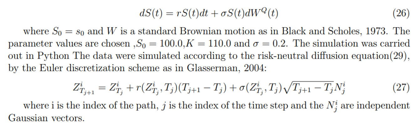
Consider the Black-Scholes model:

\

\

7.2 Hedging Experiment

This experiment begins by shorting a European call option with maturity T. The derivative will be hedged by trading the underlying asset. A ∆ hedging strategy is considered, and the portfolio consisting of positions on the underlying is rebalanced weekly, according to the newly computed ∆ weights.

\ \

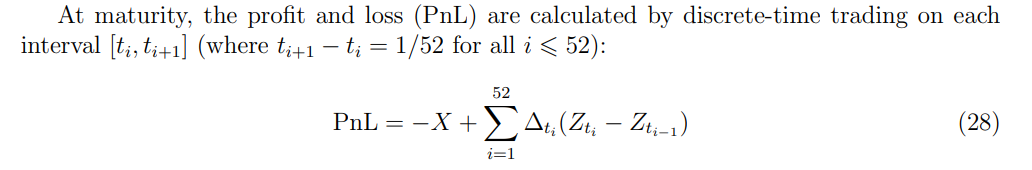
\ \ A simulation of the evolution of Z across n paths is conducted, producing n PnL values. A histogram is used to visualize the distribution of the PnL values across paths. The different methods are then subjected to this experiment, and the results are compared to the BlackScholes case.

\ The PnL values are reported relative to the portfolio value at period 0, which is the premium of the sold European call option. The relative hedging error is measured by the standard deviation of the histogram produced. This metric is widely used in evaluating the performance of different models, as in Frandsen et al., 2022.

\

7.3 Least Squares Monte Carlo Algorithm

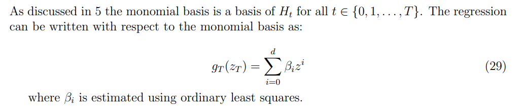
7.3.1 Monomial Basis

\ \

\ \ 7.3.2 Neural Network Basis

\ Alternatively, the regression can be conducted using a parametric basis, such as a neural network, where:

\ \

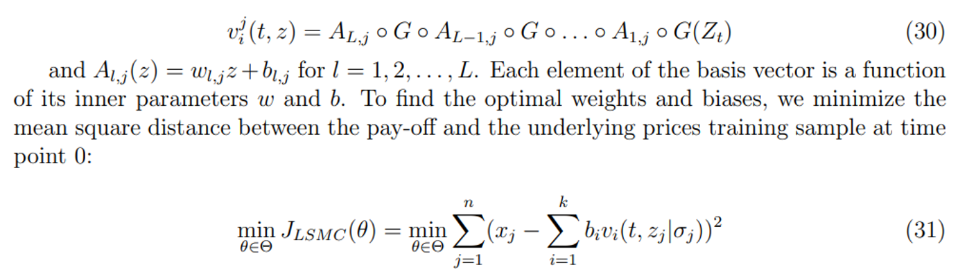
\ \ The architecture of the neural network is crucial, and a multi-layer neural network with l > 1 is preferred, as supported by Proposition 5.3 and empirical studies in various applications. In this example, the layer dimension is set to l = 4, which can be further fine-tuned for explanatory power. The back-propagation algorithm is used to update the weights and biases after each epoch, achieved by minimizing the loss function with respect to the inner parameters through stochastic gradient descent as in Kingma and Ba, 2014

\

7.4 Differential Machine Learning Algorithm

From proposition 3.4, we can infer, given the sample ((x1, z1)), . . . ,(xn, zn)), that the loss function with respect to the training sample is:

\ \

\ \ \ \ \

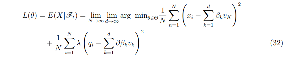
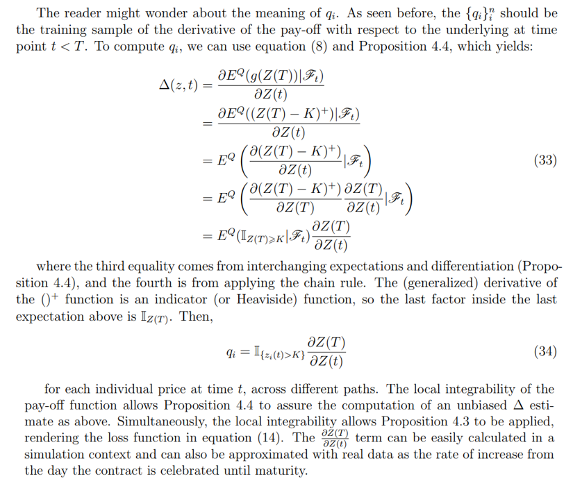
\ \ By computing qi through the simulation of at least two different paths, applying the indicator function, and averaging the resulting quantities, the ∆ hedging estimate is obtained. This method allows for efficient and accurate hedging strategies, making it a valuable tool in the field of mathematical finance.

\ 7.4.1 Neural Network basis

\ All the details of this implementation can be found in Huge and Savine, 2020. Examining equation (30), the first part is the same loss function as in the LSMC case. Still, the second part constitutes the mean square difference between the differential labels and the derivative of the entire neural network with respect to price. So, we need to obtain the derivative of the feed-forward neural network. Feed-forward neural networks are efficiently differentiated by backpropagation.

\ Then recapitulating the feed-forward equations:

\ \

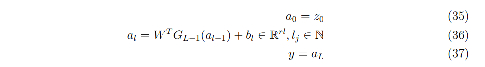
\ \ Recall that the inputs are states and the predictors are prices for the first part, hence, these differentials are predicted risk sensitivities, obtained by differentiation of the line above, in the reverse order:

\ \

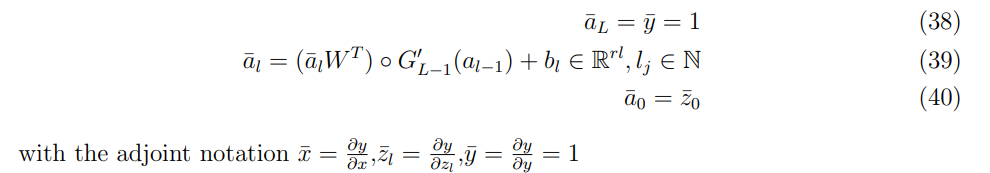
\ \ Then the implementation can be divided into the following two steps:

\

1. The neural network for the standard feed-forward equations (35)-(37) is built, paying careful attention to the use of the functionalities of software to store all intermediate values. The neural network architecture will comprehend 4 hidden layers, that is a multi-layer structure as prescribed in section 6.2.1 Note that the activation function needs to be differentiable, in order for equations (38)-(40), to be applied, so the following Huge and Savine, 2020, a soft-plus function was chosen.

   \

2. Implement as a standard function in Python the equations (35)-(37). Note that the intermediate values stored before are going to be the domain of this function.

\

1. Combine both functions in a single function, named the Twin Tower.

   \

2. Train the Twin Tower with respect to the loss equation(14).

\

:::info Author:

(1) Pedro Duarte Gomes, Department of Mathematics, University of Copenhagen.

:::

:::info This paper is available on arxiv under CC by 4.0 Deed (Attribution 4.0 International) license.

:::

\