Once you have deployed a machine learning model to production, it typically falls into one of two categories.

First, there are real-time models that need to be always available, ready to serve predictions with minimal latency. These handle requests one at a time(or in small batches), but the requests come in unpredictably throughout the day. Think fraud detection systems that need to evaluate transactions as they happen-speed is critical.

Then there are batch inference models that run on a schedule, usually processing large volumes of predictions all at once. Maybe you are generating demand forecasts for thousands of products every week, or creating monthly revenue projections across all your sales regions. These jobs don’t need instant responses, but they need to handle significant scale.

Traditionally, serverless model serving has been reserved for real-time use cases. For batch predictions, teams would typically pull a saved model from a registry and incorporate it into a data pipeline to process requests in bulk. This means a data engineer has to write expensive Python code to loop through batches, run predictions, and integrate all of that into their ETL pipelines. On top of that, they need to manage the infrastructure-spinning up clusters when needed, ensuring they are sized correctly for the workloads, and remembering to shut them down afterward to avoid unnecessary costs.

This approach also creates a barrier for SQL analysts who want to use these models directly in their queries and scripts. They end up dependent on engineering teams to run predictions for them.

To mitigate these issues, I will walk you through how to deploy models on Databricks model serving and use AI Functions to run these batch predictions. That results in zero maintenance in terms of infrastructure and enables sql analysts to incorporate model inference as part of their workflow.

Retail Sales Forecasting with Databricks Model Serving

Retail organizations need accurate sales forecasts to optimize inventory management, staffing levels and promotional planning, and supply chain operations. Traditional forecasting often requires significant manual effort from data science teams to generate predictions, creating bottlenecks when business analysts need quick insights across multiple stores, products or time horizons. Generating these forecasts required data engineers to manually run batch prediction jobs, manage compute infrastructure and create custom pipelines for each request-making the process slow, expensive and inaccessible to business users.

By transforming batch inference into a simple SQL function, we transform what was once a complex engineering tasks requiring Python expertise and infrastructure management into a simple query. In this example we will show you how to train a forecasting model on Databricks, serve it in model serving and run batch inference using AI Functions.

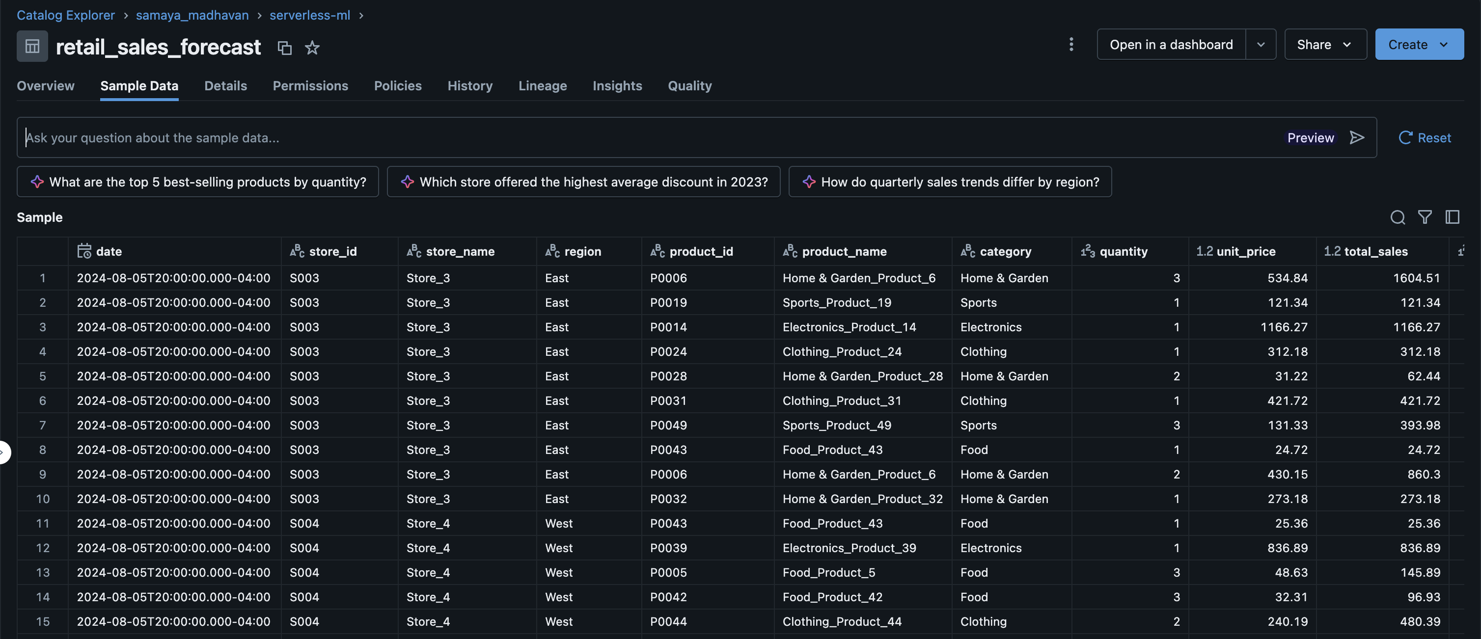
Step 1 : Create a sample fake data set that contains retail sales data with realistic patterns.

The generated dataset is a synthetic retail sales transactions dataset designed for time series forecasting. Each row represents a single sales transaction and includes the following fields:

• date: Transaction date
• storeid, storename, region: Store identifiers and region
• productid, productname, category: Product identifiers and category
• quantity: Number of units sold in the transaction
• unit_price: Price per unit (with random variation)
• total_sales: Total sales amount before discount
• discountpct, discountamount: Discount applied and its value
• final_sales: Sales amount after discount
• dayofweek, month, year, quarter: Temporal features for analysis

The dataset covers multiple years, stores, and products, and incorporates realistic retail patterns such as seasonality, holidays, promotions, and growth trends.

\

import pandas as pd import numpy as np  def generate_retail_sales_data(start_date='2021-01-01', end_date='2024-12-31',                                  num_stores=10, num_products=50, seed=42):     """Generate synthetic retail sales data with realistic patterns."""     np.random.seed(seed)      # Generate date range     date_range = pd.date_range(start=start_date, end=end_date, freq='D')      # Product categories and their base prices     categories = ['Electronics', 'Clothing', 'Food', 'Home & Garden', 'Sports']     store_regions = ['North', 'South', 'East', 'West', 'Central']      data = []      # Generate product catalog     products = []     for i in range(num_products):         category = np.random.choice(categories)         base_price = np.random.uniform(10, 500)         if category == 'Electronics':             base_price = np.random.uniform(100, 2000)         elif category == 'Food':             base_price = np.random.uniform(5, 50)          products.append({             'product_id': f'P{i+1:04d}',             'product_name': f'{category}_Product_{i+1}',             'category': category,             'base_price': base_price         })      # Generate store information     stores = []     for i in range(num_stores):         stores.append({             'store_id': f'S{i+1:03d}',             'store_name': f'Store_{i+1}',             'region': store_regions[i % len(store_regions)]         })      # Generate sales transactions     for date in date_range:         day_of_week = date.dayofweek         month = date.month          # Apply seasonal factors         weekend_factor = 1.2 if day_of_week >= 5 else 1.0  # 20% boost on weekends         holiday_factor = 1.5 if month in [11, 12] else 1.0  # 50% boost in holiday season         summer_factor = 0.85 if month in [6, 7, 8] else 1.0  # 15% slowdown in summer          # Apply growth trend (5% annual growth)         days_since_start = (date - pd.Timestamp(start_date)).days         trend_factor = 1 + (days_since_start / 365) * 0.05          # Generate transactions for each store         for store in stores:             store_factor = np.random.uniform(0.7, 1.3)              # Calculate number of transactions for this store on this day             base_transactions = int(np.random.poisson(15) * weekend_factor *                                     holiday_factor * summer_factor *                                     trend_factor * store_factor)              for _ in range(base_transactions):                 product = np.random.choice(products)                  # Quantity sold per transaction                 quantity = np.random.choice([1, 2, 3, 4, 5],                                             p=[0.5, 0.25, 0.15, 0.07, 0.03])                  # Apply price variation (promotions, dynamic pricing)                 price_variation = np.random.uniform(0.85, 1.15)                 unit_price = product['base_price'] * price_variation                  # Calculate sales amounts                 total_sales = unit_price * quantity                  # Apply discounts                 discount_pct = np.random.choice([0, 5, 10, 15, 20],                                                 p=[0.6, 0.2, 0.1, 0.07, 0.03])                 discount_amount = total_sales * (discount_pct / 100)                 final_sales = total_sales - discount_amount                  # Append transaction record                 data.append({                     'date': date,                     'store_id': store['store_id'],                     'store_name': store['store_name'],                     'region': store['region'],                     'product_id': product['product_id'],                     'product_name': product['product_name'],                     'category': product['category'],                     'quantity': quantity,                     'unit_price': round(unit_price, 2),                     'total_sales': round(total_sales, 2),                     'discount_pct': discount_pct,                     'discount_amount': round(discount_amount, 2),                     'final_sales': round(final_sales, 2),                     'day_of_week': date.day_name(),                     'month': date.month,                     'year': date.year,                     'quarter': f'Q{(date.month-1)//3 + 1}'                 })      df = pd.DataFrame(data)     return df   def save_to_unity_catalog(df, catalog_name, schema_name, table_name):     """Save DataFrame to Unity Catalog as a Delta table."""     spark_df = spark.createDataFrame(df)      # Handle schema names with hyphens     if "-" in schema_name:         schema_name = f"`{schema_name}`"      full_table_name = f"{catalog_name}.{schema_name}.{table_name}"      # Write as Delta table     spark_df.write \         .format("delta") \         .mode("overwrite") \         .option("overwriteSchema", "true") \         .saveAsTable(full_table_name)      return full_table_name   # Generate retail sales data sales_df = generate_retail_sales_data(     start_date='2021-01-01',     end_date='2024-12-31',     num_stores=10,     num_products=50,     seed=42 )  # Configure Unity Catalog location catalog = "samaya_madhavan" schema = "serverless-ml" table = "retail_sales_forecast"  # Save to Unity Catalog table_path = save_to_unity_catalog(sales_df, catalog, schema, table)  # Display summary print(f"Generated {len(sales_df):,} transaction records") print(f"Date range: {sales_df['date'].min()} to {sales_df['date'].max()}") print(f"Total sales: ${sales_df['final_sales'].sum():,.2f}") print(f"Data saved to: {table_path}") 

The output of this is saved to unity catalog :

Step 2 : Build, register and deploy a time series forecasting model.

The next step in the process is to build, register and deploy a time series forecasting model using scikit-learn’s LinearRegression, with MLFlow for model management and Databricks Model Serving for deployment.

We start by loading and preparing retail sales data from the unity catalog table, aggregating daily sales for a specific store. The data is split into training and test sets, and features such as day index, day of week, and month are engineered for the model. A LinearRegression model is trained, evaluated, and logged to MLflow along with a StandardScaler for feature normalization.

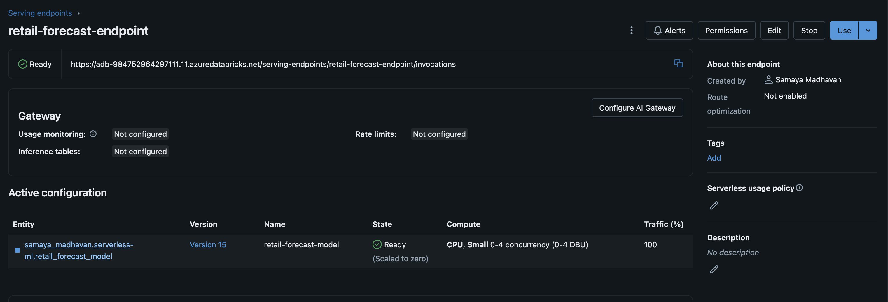
A custom MLflow pyfunc wrapper is then created to enable multi-period forecasting, and the model is registered in Unity Catalog. The notebook proceeds to deploy the model to a Databricks Model Serving endpoint.

import pandas as pd import numpy as np import mlflow import mlflow.sklearn from sklearn.linear_model import LinearRegression from sklearn.preprocessing import StandardScaler from mlflow.models import infer_signature  # Configuration catalog = "samaya_madhavan" schema = "serverless-ml" source_table = "retail_sales_forecast" model_name = f"{catalog}.{schema}.retail_forecast_model" endpoint_name = "retail-forecast-endpoint"  # Step 1: Load and prepare data print("Loading data...") df = spark.sql(f"""   SELECT     date,     SUM(final_sales) AS sales   FROM {catalog}.`{schema}`.{source_table}   WHERE store_id = 'S001'   GROUP BY date   ORDER BY date """).toPandas()  df['date'] = pd.to_datetime(df['date']) df['day_index'] = (df['date'] - df['date'].min()).dt.days df['day_of_week'] = df['date'].dt.dayofweek df['month'] = df['date'].dt.month  # Create train/test split train_size = int(len(df) * 0.8) train_df = df[:train_size] test_df = df[train_size:]  X_train = train_df[['day_index', 'day_of_week', 'month']] y_train = train_df['sales'] X_test = test_df[['day_index', 'day_of_week', 'month']] y_test = test_df['sales']  print(f"Training samples: {len(X_train)}, Test samples: {len(X_test)}")  # Step 2: Train sklearn model print("\nTraining LinearRegression model...") mlflow.set_registry_uri("databricks-uc")  with mlflow.start_run(run_name="sklearn_forecast") as run:     # Train scaler and model     scaler = StandardScaler()     X_train_scaled = scaler.fit_transform(X_train)     X_test_scaled = scaler.transform(X_test)      model = LinearRegression()     model.fit(X_train_scaled, y_train)      # Evaluate     train_score = model.score(X_train_scaled, y_train)     test_score = model.score(X_test_scaled, y_test)      print(f"Train R²: {train_score:.4f}")     print(f"Test R²: {test_score:.4f}")      # Log metrics     mlflow.log_metric("train_r2", train_score)     mlflow.log_metric("test_r2", test_score)      # Save scaler separately     import joblib     joblib.dump(scaler, "/tmp/scaler.pkl")     mlflow.log_artifact("/tmp/scaler.pkl")      # Create input/output examples for signature     input_example = pd.DataFrame({'periods': [30]})      # Generate sample forecast     last_day = df['day_index'].max()     last_date = df['date'].max()     forecast_rows = []      for i in range(1, 6):  # Sample 5 days         future_date = last_date + pd.Timedelta(days=i)         future_day = last_day + i         X_future = pd.DataFrame([{             'day_index': future_day,             'day_of_week': future_date.dayofweek,             'month': future_date.month         }])         X_future_scaled = scaler.transform(X_future)         pred = model.predict(X_future_scaled)[0]          forecast_rows.append({             'date': future_date.strftime('%Y-%m-%d'),             'forecast': float(pred),             'forecast_lower': float(pred * 0.9),             'forecast_upper': float(pred * 1.1)         })      output_example = pd.DataFrame(forecast_rows)     signature = infer_signature(input_example, output_example)      # Log model with sklearn flavor     mlflow.sklearn.log_model(         sk_model=model,         artifact_path="model",         signature=signature,         input_example=input_example,         registered_model_name=model_name,         serialization_format="cloudpickle"     )      print(f"\nModel registered: {model_name}")  # Step 3: Create wrapper model for forecasting print("\nCreating forecast wrapper...")  with mlflow.start_run(run_name="sklearn_forecast_wrapper") as run:     class SklearnForecastWrapper(mlflow.pyfunc.PythonModel):         def load_context(self, context):             import joblib             self.model = joblib.load(context.artifacts["model"])             self.scaler = joblib.load(context.artifacts["scaler"])             self.last_day_index = int(open(context.artifacts["last_day"]).read())             self.last_date = pd.to_datetime(open(context.artifacts["last_date"]).read())          def predict(self, context, model_input):             if isinstance(model_input, pd.DataFrame) and 'periods' in model_input.columns:                 periods = int(model_input['periods'].iloc[0])             else:                 periods = 30              forecasts = []             for i in range(1, periods + 1):                 future_date = self.last_date + pd.Timedelta(days=i)                 future_day = self.last_day_index + i                  X_future = pd.DataFrame([{                     'day_index': future_day,                     'day_of_week': future_date.dayofweek,                     'month': future_date.month                 }])                  X_scaled = self.scaler.transform(X_future)                 pred = self.model.predict(X_scaled)[0]                  forecasts.append({                     'date': future_date.strftime('%Y-%m-%d'),                     'forecast': float(pred),                     'forecast_lower': float(pred * 0.9),                     'forecast_upper': float(pred * 1.1)                 })              # Return in ai_query compatible format - single element array             return pd.DataFrame([{"predictions": forecasts}])      # Save artifacts     import joblib     joblib.dump(model, "/tmp/sklearn_model.pkl")     joblib.dump(scaler, "/tmp/sklearn_scaler.pkl")      with open("/tmp/last_day.txt", "w") as f:         f.write(str(int(last_day)))      with open("/tmp/last_date.txt", "w") as f:         f.write(str(last_date))      # Create signature     input_example = pd.DataFrame({'periods': [30]})     wrapper = SklearnForecastWrapper()     wrapper.model = model     wrapper.scaler = scaler     wrapper.last_day_index = int(last_day)     wrapper.last_date = last_date     output_example = wrapper.predict(None, input_example)     signature = infer_signature(input_example, output_example)      # Log wrapper model     mlflow.pyfunc.log_model(         artifact_path="model",         python_model=SklearnForecastWrapper(),         artifacts={             "model": "/tmp/sklearn_model.pkl",             "scaler": "/tmp/sklearn_scaler.pkl",             "last_day": "/tmp/last_day.txt",             "last_date": "/tmp/last_date.txt"         },         signature=signature,         input_example=input_example,         registered_model_name=model_name     )      print(f"Wrapper model registered: {model_name}")  # Step 4: Get latest version and set alias from mlflow.tracking import MlflowClient client = MlflowClient()  model_versions = client.search_model_versions(f"name='{model_name}'") latest_version = max([int(mv.version) for mv in model_versions])  client.set_registered_model_alias(model_name, "Champion", str(latest_version)) print(f"\nLatest version: {latest_version} (alias: Champion)")  # Step 5: Deploy to Model Serving print("\nDeploying to Model Serving...") from mlflow.deployments import get_deploy_client  deploy_client = get_deploy_client("databricks")  endpoint_config = {     "served_entities": [{         "name": "retail-forecast-model",         "entity_name": model_name,         "entity_version": str(latest_version),         "workload_size": "Small",         "scale_to_zero_enabled": True     }],     "traffic_config": {         "routes": [{"served_model_name": "retail-forecast-model", "traffic_percentage": 100}]     } }  try:     deploy_client.get_endpoint(endpoint=endpoint_name)     deploy_client.update_endpoint(endpoint=endpoint_name, config=endpoint_config)     print(f"✓ Updated endpoint: {endpoint_name}") except:     deploy_client.create_endpoint(name=endpoint_name, config=endpoint_config)     print(f"✓ Created endpoint: {endpoint_name}")  # Step 6: Test the endpoint print("\nTesting endpoint...") import time time.sleep(10)  try:     result = deploy_client.predict(         endpoint=endpoint_name,         inputs={"dataframe_records": [{"periods": 7}]}     )     print("\nSample forecast (7 days):")     if isinstance(result, dict) and 'predictions' in result:         print(pd.DataFrame(result['predictions']).head())     else:         print(result) except Exception as e:     print(f"Endpoint may still be starting: {e}")  print(f"\n{'='*60}") print(f"Deployment Complete!") print(f"{'='*60}") print(f"Model: {model_name}") print(f"Version: {latest_version}") print(f"Endpoint: {endpoint_name}") 

The model is now served on Databricks Model Serving

\

Step 3 : Use AI Functions to obtain forecasts from the model served on Model Serving.

Finally, we demonstrate how to use AI Functions to run batch predictions.

AI Functions : Databricks offers AI Functions as native, ready-to-use capabilities that enable you to perform AI operations-such as translating text or analyzing sentiment-directly on data stored within the Databricks platform. These functions are accessible across the entire Databricks ecosystem, including SQL environments, notebooks, Lakeflow Declarative Pipelines, and Workflows.

The AI Functions catalog includes two categories :

Specialized functions deliver targeted AI capabilities for specific use cases, such as text summarization and language translation. These functions utilize cutting-edge generative AI models that Databricks hosts and maintains.

General purpose functions:ai_query() serves as a flexible, multi-purpose function that enables you to apply virtually any AI model to your datasets.

In this blog we will show you examples of how to use aiquery(). The following code shows how to use the SQL aiquery() function to obtain forecasts from the deployed Model Serving endpoint on Databricks.

Example 1: 30 day forecast.

forecast_30 = spark.sql(f""" SELECT ai_query( '{endpoint_name}', named_struct('periods', 30) ) AS forecast_json """) display(forecast_30) 

Example 2: Multiple forecast horizons

multi_forecast = spark.sql(f"""  SELECT horizon, days, ai_query( '{endpoint_name}', named_struct('periods', days) ) AS forecast_json  FROM ( SELECT 'Short-term' AS horizon, 7 AS days  UNION ALL SELECT 'Medium-term' AS horizon, 30 AS days UNION ALL SELECT 'Long-term' AS horizon, 90 AS days ) """) 

Example 3: Generate forecasts for all stores

source_table = "retail_sales_forecast"  # Get list of all stores stores = spark.sql(f"""   SELECT DISTINCT store_id, region   FROM {catalog}.`{schema}`.{source_table}   ORDER BY store_id """)  display(stores)  # Create batch forecast requests batch_requests = spark.sql(f"""   CREATE OR REPLACE TABLE {catalog}.`{schema}`.batch_forecast_requests AS   SELECT      store_id,     region,     30 AS forecast_periods,     CURRENT_TIMESTAMP() AS request_timestamp   FROM (     SELECT DISTINCT store_id, region     FROM {catalog}.`{schema}`.{source_table}   ) """)  print("✓ Batch requests table created")  # Execute batch forecasts using ai_query batch_forecasts = spark.sql(f"""   CREATE OR REPLACE TABLE {catalog}.`{schema}`.batch_forecasts AS   SELECT      r.store_id,     r.region,     r.forecast_periods,     r.request_timestamp,     pred.date AS forecast_date,     pred.forecast AS predicted_sales,     pred.forecast_lower,     pred.forecast_upper   FROM {catalog}.`{schema}`.batch_forecast_requests r   LATERAL VIEW explode(     ai_query(       '{endpoint_name}',       named_struct('periods', r.forecast_periods)     ).predictions   ) AS pred """)  print("✓ Batch forecasts completed and saved")  # View results results = spark.sql(f"""   SELECT *   FROM {catalog}.`{schema}`.batch_forecasts   ORDER BY store_id, forecast_date   LIMIT 50 """)  display(results) 

\ By deploying our retail sales forecasting model to Databricks Model Serving and leveraging AI Functions, we eliminated the need for data engineers to write custom Python loops, manage cluster infrastructure, or worry about scaling batch prediction workloads. SQL analysts can now generate 30-day forecasts for a single store, compare short-term versus long-term predictions, or produce forecasts across all ten stores in our retail chain—all with simple SQL queries using ai_query(). By bridging the gap between model deployment and data analysis, AI Functions don't just simplify batch inference—they democratize it. This is the paradigm shift that makes AI truly accessible: when running predictions becomes as simple as writing a WHERE clause, organizations can finally unlock intelligence from their data at the speed of thought rather than the speed of engineering sprints.

\