

AI Learns to Predict Shock Waves
Table of Links
Abstract and 1. Introduction
1.1. Introductory remarks
1.2. Basics of neural networks
1.3. About the entropy of direct PINN methods
1.4. Organization of the paper
-
Non-diffusive neural network solver for one dimensional scalar HCLs
2.1. One shock wave
2.2. Arbitrary number of shock waves
2.3. Shock wave generation
2.4. Shock wave interaction
2.5. Non-diffusive neural network solver for one dimensional systems of CLs
2.6. Efficient initial wave decomposition
-
Gradient descent algorithm and efficient implementation
3.1. Classical gradient descent algorithm for HCLs
3.2. Gradient descent and domain decomposition methods
-
Numerics
4.1. Practical implementations
4.2. Basic tests and convergence for 1 and 2 shock wave problems
4.3. Shock wave generation
4.4. Shock-Shock interaction
4.5. Entropy solution
4.6. Domain decomposition
4.7. Nonlinear systems
-
Conclusion and References
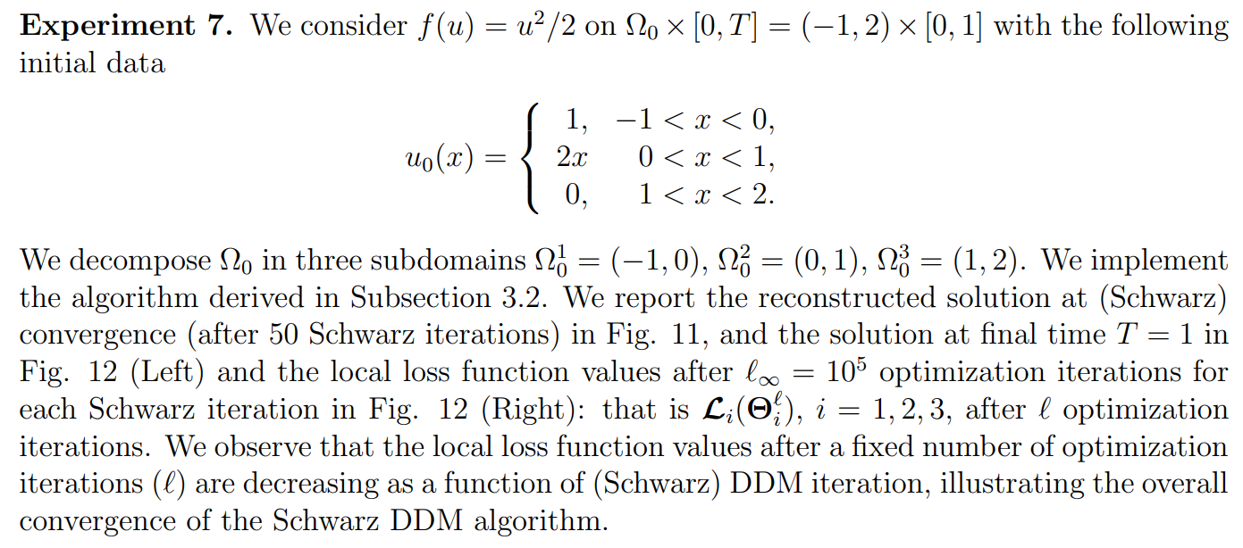
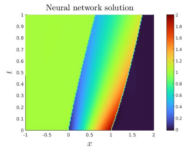
4.6. Domain decomposition
In this subsection, we propose an experiment illustrating the combination of the neural network based HCL solver developed in this paper with the domain decomposition method from Subsection 3.2. We numerically illustrate the convergence of the algorithm. The neural networks have 30 neurons and one hidden layer, and the number of learning nodes is 900 learning nodes.
\ 
\ 
\ 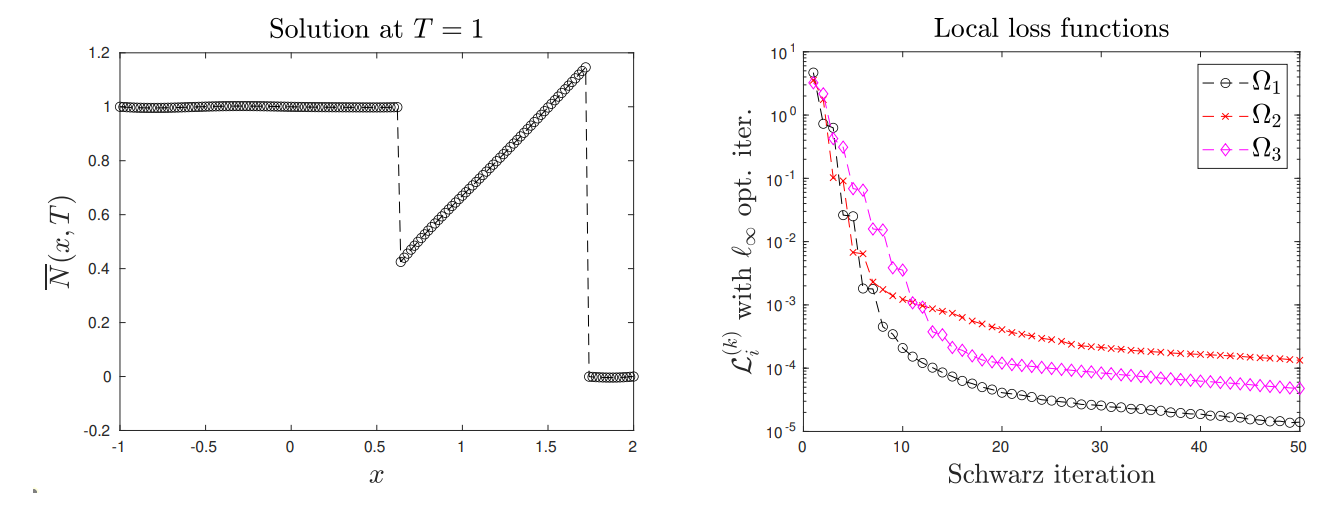
\ The DDM naturally makes sense for much more computationally complex problems. This test however illustrates a proof-of-concept of the SWR approach.
4.7. Nonlinear systems
In this subsection, we are interested in the numerical approximation of hyperbolic systems with shock waves.
\ Experiment 8. In this experiment we focus on the initial wave decomposition for a Riemann problem. The system considered here is the Shallow water equations (m = 2).
\ \ 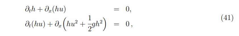
\ \ where h is the height of a compressible fluid, u its velocity, and g is the gravitational constant taken here equal to 1. The spatial domain is (−0.1, 0.1), the final time is T = 0.0025, and we impose null Dirichlet boundary conditions.
\ Experiment 8a. The initial data is given by
\ \ 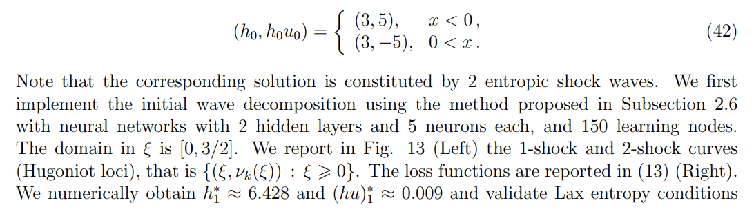
\ \ \ 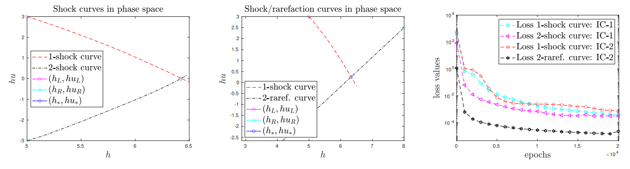
\ \ \ 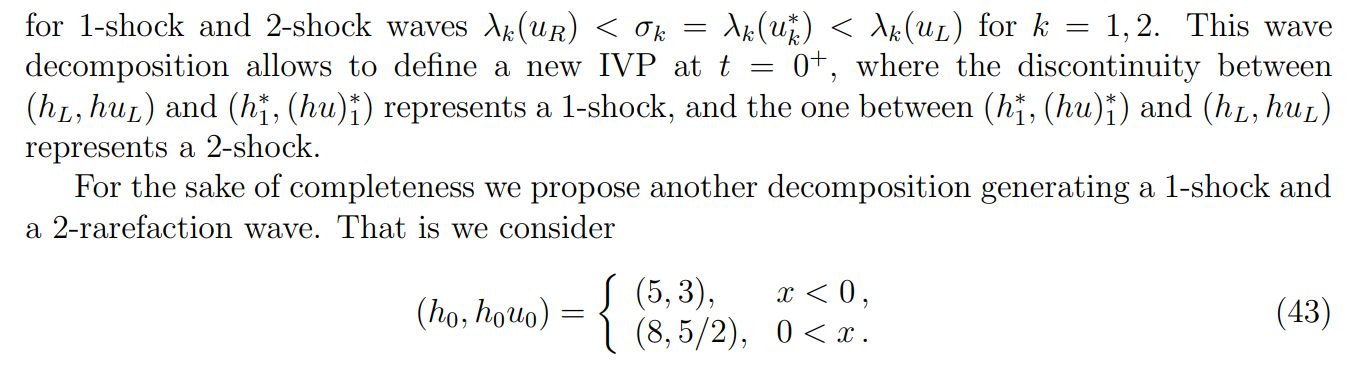
\ \ \ 
\ \ \ 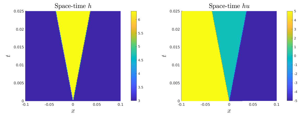
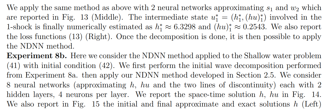
\ \ and hu (Middle), as well as the loss function Fig. 15 (Right). This experiment shows that
\ \ 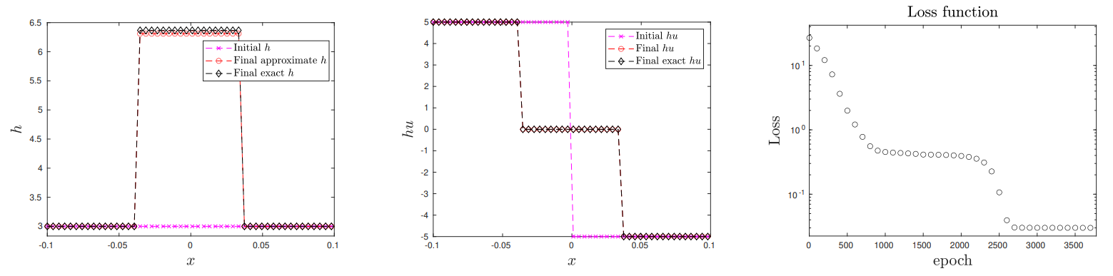
\ \ the proposed methodology allows for the computation of the solution to (at least simple) Riemann problems.
\ Experiment 9. In this last experiment, we consider Euler’s equations modeling compressible inviscid fluid flows. This is a 3-equation HCL which reads as follows (in conservative form)
\ \ 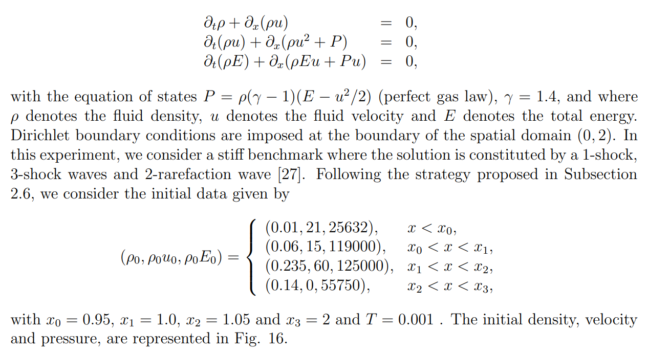
\ \ \ 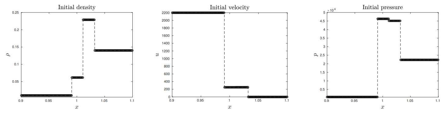
\ \ We implement the method developed in Subsection 2.5 with m = 3, 1 hidden layer and 30 neurons for each conservative component ρ, ρu, ρE and for the 3 lines of discontinuity. In Fig. 17 we report the density, velocity and pressure at initial and final times T. This test illustrates the precision of the proposed approach, with in particular an accurate approximation of the 2-contact discontinuity which is often hard to obtain with standard solvers.
\
:::info Authors:
(1) Emmanuel LORIN, School of Mathematics and Statistics, Carleton University, Ottawa, Canada, K1S 5B6 and Centre de Recherches Mathematiques, Universit´e de Montr´eal, Montreal, Canada, H3T 1J4 (elorin@math.carleton.ca);
(2) Arian NOVRUZI, a Corresponding Author from Department of Mathematics and Statistics, University of Ottawa, Ottawa, ON K1N 6N5, Canada (novruzi@uottawa.ca).
:::
:::info This paper is available on arxiv under CC by 4.0 Deed (Attribution 4.0 International) license.
:::
\
Ayrıca Şunları da Beğenebilirsiniz

Those Who Missed XRP Now Eye Apeing ($APEING) as One of 2025’s Next Crypto to Hit $1

Polygon Tops RWA Rankings With $1.1B in Tokenized Assets

