Try This if Your TensorFlow Code Is Slow
Content Overview
- Overview
- Setup
- Taking advantage of graphs
- Using tf.function
- Seeing the speed-up
- When is a tf.function tracing?
- Next steps
\
Overview
This guide goes beneath the surface of TensorFlow and Keras to demonstrate how TensorFlow works. If you instead want to immediately get started with Keras, check out the collection of Keras guides.
In this guide, you'll learn how TensorFlow allows you to make simple changes to your code to get graphs, how graphs are stored and represented, and how you can use them to accelerate your models.
\
:::tip Note: For those of you who are only familiar with TensorFlow 1.x, this guide demonstrates a very different view of graphs.
:::
This is a big-picture overview that covers how tf.function allows you to switch from eager execution to graph execution. For a more complete specification of tf.function, go to the Better performance with tf.function guide.
What are graphs?
In the previous three guides, you ran TensorFlow eagerly. This means TensorFlow operations are executed by Python, operation by operation, and return results back to Python.
While eager execution has several unique advantages, graph execution enables portability outside Python and tends to offer better performance. Graph execution means that tensor computations are executed as a TensorFlow graph, sometimes referred to as a tf.Graph or simply a "graph."
Graphs are data structures that contain a set of tf.Operation objects, which represent units of computation; and tf.Tensor objects, which represent the units of data that flow between operations. They are defined in a tf.Graph context. Since these graphs are data structures, they can be saved, run, and restored all without the original Python code.
This is what a TensorFlow graph representing a two-layer neural network looks like when visualized in TensorBoard:
\n 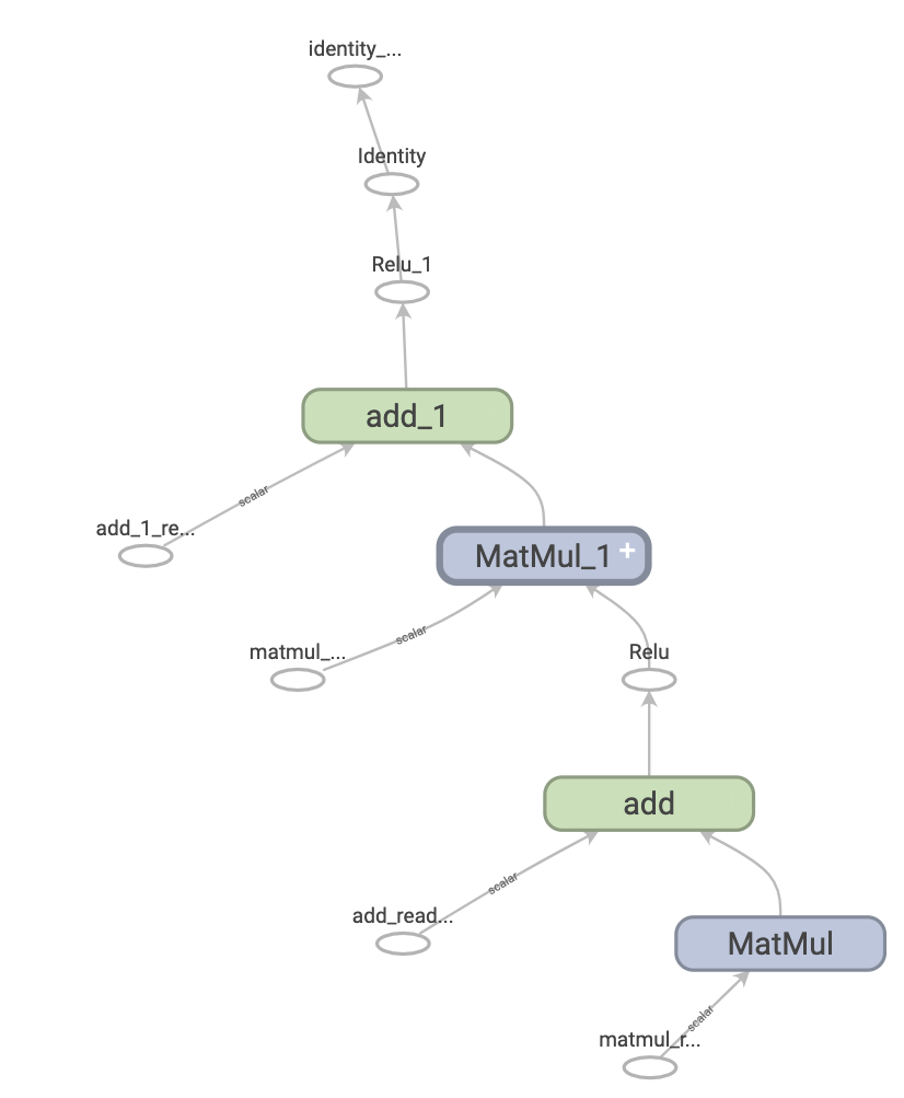
The benefits of graphs
With a graph, you have a great deal of flexibility. You can use your TensorFlow graph in environments that don't have a Python interpreter, like mobile applications, embedded devices, and backend servers. TensorFlow uses graphs as the format for saved models when it exports them from Python.
Graphs are also easily optimized, allowing the compiler to do transformations like:
- Statically infer the value of tensors by folding constant nodes in your computation ("constant folding").
- Separate sub-parts of a computation that are independent and split them between threads or devices.
- Simplify arithmetic operations by eliminating common subexpressions.
There is an entire optimization system, Grappler, to perform this and other speedups.
In short, graphs are extremely useful and let your TensorFlow run fast, run in parallel, and run efficiently on multiple devices.
However, you still want to define your machine learning models (or other computations) in Python for convenience, and then automatically construct graphs when you need them.
Setup
Import some necessary libraries:
\
import tensorflow as tf import timeit from datetime import datetime \
2024-08-15 01:23:58.511668: E external/local_xla/xla/stream_executor/cuda/cuda_fft.cc:485] Unable to register cuFFT factory: Attempting to register factory for plugin cuFFT when one has already been registered 2024-08-15 01:23:58.532403: E external/local_xla/xla/stream_executor/cuda/cuda_dnn.cc:8454] Unable to register cuDNN factory: Attempting to register factory for plugin cuDNN when one has already been registered 2024-08-15 01:23:58.538519: E external/local_xla/xla/stream_executor/cuda/cuda_blas.cc:1452] Unable to register cuBLAS factory: Attempting to register factory for plugin cuBLAS when one has already been registered Taking advantage of graphs
You create and run a graph in TensorFlow by using tf.function, either as a direct call or as a decorator. tf.function takes a regular function as input and returns a tf.types.experimental.PolymorphicFunction. A PolymorphicFunction is a Python callable that builds TensorFlow graphs from the Python function. You use a tf.function in the same way as its Python equivalent.
\
# Define a Python function. def a_regular_function(x, y, b): x = tf.matmul(x, y) x = x + b return x # The Python type of `a_function_that_uses_a_graph` will now be a # `PolymorphicFunction`. a_function_that_uses_a_graph = tf.function(a_regular_function) # Make some tensors. x1 = tf.constant([[1.0, 2.0]]) y1 = tf.constant([[2.0], [3.0]]) b1 = tf.constant(4.0) orig_value = a_regular_function(x1, y1, b1).numpy() # Call a `tf.function` like a Python function. tf_function_value = a_function_that_uses_a_graph(x1, y1, b1).numpy() assert(orig_value == tf_function_value) \
WARNING: All log messages before absl::InitializeLog() is called are written to STDERR I0000 00:00:1723685041.078349 10585 cuda_executor.cc:1015] successful NUMA node read from SysFS had negative value (-1), but there must be at least one NUMA node, so returning NUMA node zero. See more at https://github.com/torvalds/linux/blob/v6.0/Documentation/ABI/testing/sysfs-bus-pci#L344-L355 I0000 00:00:1723685041.081709 10585 cuda_executor.cc:1015] successful NUMA node read from SysFS had negative value (-1), but there must be at least one NUMA node, so returning NUMA node zero. See more at https://github.com/torvalds/linux/blob/v6.0/Documentation/ABI/testing/sysfs-bus-pci#L344-L355 I0000 00:00:1723685041.084876 10585 cuda_executor.cc:1015] successful NUMA node read from SysFS had negative value (-1), but there must be at least one NUMA node, so returning NUMA node zero. See more at https://github.com/torvalds/linux/blob/v6.0/Documentation/ABI/testing/sysfs-bus-pci#L344-L355 I0000 00:00:1723685041.088691 10585 cuda_executor.cc:1015] successful NUMA node read from SysFS had negative value (-1), but there must be at least one NUMA node, so returning NUMA node zero. See more at https://github.com/torvalds/linux/blob/v6.0/Documentation/ABI/testing/sysfs-bus-pci#L344-L355 I0000 00:00:1723685041.100124 10585 cuda_executor.cc:1015] successful NUMA node read from SysFS had negative value (-1), but there must be at least one NUMA node, so returning NUMA node zero. See more at https://github.com/torvalds/linux/blob/v6.0/Documentation/ABI/testing/sysfs-bus-pci#L344-L355 I0000 00:00:1723685041.103158 10585 cuda_executor.cc:1015] successful NUMA node read from SysFS had negative value (-1), but there must be at least one NUMA node, so returning NUMA node zero. See more at https://github.com/torvalds/linux/blob/v6.0/Documentation/ABI/testing/sysfs-bus-pci#L344-L355 I0000 00:00:1723685041.106072 10585 cuda_executor.cc:1015] successful NUMA node read from SysFS had negative value (-1), but there must be at least one NUMA node, so returning NUMA node zero. See more at https://github.com/torvalds/linux/blob/v6.0/Documentation/ABI/testing/sysfs-bus-pci#L344-L355 I0000 00:00:1723685041.109491 10585 cuda_executor.cc:1015] successful NUMA node read from SysFS had negative value (-1), but there must be at least one NUMA node, so returning NUMA node zero. See more at https://github.com/torvalds/linux/blob/v6.0/Documentation/ABI/testing/sysfs-bus-pci#L344-L355 I0000 00:00:1723685041.112991 10585 cuda_executor.cc:1015] successful NUMA node read from SysFS had negative value (-1), but there must be at least one NUMA node, so returning NUMA node zero. See more at https://github.com/torvalds/linux/blob/v6.0/Documentation/ABI/testing/sysfs-bus-pci#L344-L355 I0000 00:00:1723685041.115870 10585 cuda_executor.cc:1015] successful NUMA node read from SysFS had negative value (-1), but there must be at least one NUMA node, so returning NUMA node zero. See more at https://github.com/torvalds/linux/blob/v6.0/Documentation/ABI/testing/sysfs-bus-pci#L344-L355 I0000 00:00:1723685041.118785 10585 cuda_executor.cc:1015] successful NUMA node read from SysFS had negative value (-1), but there must be at least one NUMA node, so returning NUMA node zero. See more at https://github.com/torvalds/linux/blob/v6.0/Documentation/ABI/testing/sysfs-bus-pci#L344-L355 I0000 00:00:1723685041.122189 10585 cuda_executor.cc:1015] successful NUMA node read from SysFS had negative value (-1), but there must be at least one NUMA node, so returning NUMA node zero. See more at https://github.com/torvalds/linux/blob/v6.0/Documentation/ABI/testing/sysfs-bus-pci#L344-L355 I0000 00:00:1723685042.369900 10585 cuda_executor.cc:1015] successful NUMA node read from SysFS had negative value (-1), but there must be at least one NUMA node, so returning NUMA node zero. See more at https://github.com/torvalds/linux/blob/v6.0/Documentation/ABI/testing/sysfs-bus-pci#L344-L355 I0000 00:00:1723685042.372045 10585 cuda_executor.cc:1015] successful NUMA node read from SysFS had negative value (-1), but there must be at least one NUMA node, so returning NUMA node zero. See more at https://github.com/torvalds/linux/blob/v6.0/Documentation/ABI/testing/sysfs-bus-pci#L344-L355 I0000 00:00:1723685042.374040 10585 cuda_executor.cc:1015] successful NUMA node read from SysFS had negative value (-1), but there must be at least one NUMA node, so returning NUMA node zero. See more at https://github.com/torvalds/linux/blob/v6.0/Documentation/ABI/testing/sysfs-bus-pci#L344-L355 I0000 00:00:1723685042.376123 10585 cuda_executor.cc:1015] successful NUMA node read from SysFS had negative value (-1), but there must be at least one NUMA node, so returning NUMA node zero. See more at https://github.com/torvalds/linux/blob/v6.0/Documentation/ABI/testing/sysfs-bus-pci#L344-L355 I0000 00:00:1723685042.378174 10585 cuda_executor.cc:1015] successful NUMA node read from SysFS had negative value (-1), but there must be at least one NUMA node, so returning NUMA node zero. See more at https://github.com/torvalds/linux/blob/v6.0/Documentation/ABI/testing/sysfs-bus-pci#L344-L355 I0000 00:00:1723685042.380184 10585 cuda_executor.cc:1015] successful NUMA node read from SysFS had negative value (-1), but there must be at least one NUMA node, so returning NUMA node zero. See more at https://github.com/torvalds/linux/blob/v6.0/Documentation/ABI/testing/sysfs-bus-pci#L344-L355 I0000 00:00:1723685042.382098 10585 cuda_executor.cc:1015] successful NUMA node read from SysFS had negative value (-1), but there must be at least one NUMA node, so returning NUMA node zero. See more at https://github.com/torvalds/linux/blob/v6.0/Documentation/ABI/testing/sysfs-bus-pci#L344-L355 I0000 00:00:1723685042.384064 10585 cuda_executor.cc:1015] successful NUMA node read from SysFS had negative value (-1), but there must be at least one NUMA node, so returning NUMA node zero. See more at https://github.com/torvalds/linux/blob/v6.0/Documentation/ABI/testing/sysfs-bus-pci#L344-L355 I0000 00:00:1723685042.386002 10585 cuda_executor.cc:1015] successful NUMA node read from SysFS had negative value (-1), but there must be at least one NUMA node, so returning NUMA node zero. See more at https://github.com/torvalds/linux/blob/v6.0/Documentation/ABI/testing/sysfs-bus-pci#L344-L355 I0000 00:00:1723685042.387981 10585 cuda_executor.cc:1015] successful NUMA node read from SysFS had negative value (-1), but there must be at least one NUMA node, so returning NUMA node zero. See more at https://github.com/torvalds/linux/blob/v6.0/Documentation/ABI/testing/sysfs-bus-pci#L344-L355 I0000 00:00:1723685042.389902 10585 cuda_executor.cc:1015] successful NUMA node read from SysFS had negative value (-1), but there must be at least one NUMA node, so returning NUMA node zero. See more at https://github.com/torvalds/linux/blob/v6.0/Documentation/ABI/testing/sysfs-bus-pci#L344-L355 I0000 00:00:1723685042.391922 10585 cuda_executor.cc:1015] successful NUMA node read from SysFS had negative value (-1), but there must be at least one NUMA node, so returning NUMA node zero. See more at https://github.com/torvalds/linux/blob/v6.0/Documentation/ABI/testing/sysfs-bus-pci#L344-L355 I0000 00:00:1723685042.431010 10585 cuda_executor.cc:1015] successful NUMA node read from SysFS had negative value (-1), but there must be at least one NUMA node, so returning NUMA node zero. See more at https://github.com/torvalds/linux/blob/v6.0/Documentation/ABI/testing/sysfs-bus-pci#L344-L355 I0000 00:00:1723685042.433093 10585 cuda_executor.cc:1015] successful NUMA node read from SysFS had negative value (-1), but there must be at least one NUMA node, so returning NUMA node zero. See more at https://github.com/torvalds/linux/blob/v6.0/Documentation/ABI/testing/sysfs-bus-pci#L344-L355 I0000 00:00:1723685042.435050 10585 cuda_executor.cc:1015] successful NUMA node read from SysFS had negative value (-1), but there must be at least one NUMA node, so returning NUMA node zero. See more at https://github.com/torvalds/linux/blob/v6.0/Documentation/ABI/testing/sysfs-bus-pci#L344-L355 I0000 00:00:1723685042.437074 10585 cuda_executor.cc:1015] successful NUMA node read from SysFS had negative value (-1), but there must be at least one NUMA node, so returning NUMA node zero. See more at https://github.com/torvalds/linux/blob/v6.0/Documentation/ABI/testing/sysfs-bus-pci#L344-L355 I0000 00:00:1723685042.439053 10585 cuda_executor.cc:1015] successful NUMA node read from SysFS had negative value (-1), but there must be at least one NUMA node, so returning NUMA node zero. See more at https://github.com/torvalds/linux/blob/v6.0/Documentation/ABI/testing/sysfs-bus-pci#L344-L355 I0000 00:00:1723685042.441049 10585 cuda_executor.cc:1015] successful NUMA node read from SysFS had negative value (-1), but there must be at least one NUMA node, so returning NUMA node zero. See more at https://github.com/torvalds/linux/blob/v6.0/Documentation/ABI/testing/sysfs-bus-pci#L344-L355 I0000 00:00:1723685042.442965 10585 cuda_executor.cc:1015] successful NUMA node read from SysFS had negative value (-1), but there must be at least one NUMA node, so returning NUMA node zero. See more at https://github.com/torvalds/linux/blob/v6.0/Documentation/ABI/testing/sysfs-bus-pci#L344-L355 I0000 00:00:1723685042.444941 10585 cuda_executor.cc:1015] successful NUMA node read from SysFS had negative value (-1), but there must be at least one NUMA node, so returning NUMA node zero. See more at https://github.com/torvalds/linux/blob/v6.0/Documentation/ABI/testing/sysfs-bus-pci#L344-L355 I0000 00:00:1723685042.446890 10585 cuda_executor.cc:1015] successful NUMA node read from SysFS had negative value (-1), but there must be at least one NUMA node, so returning NUMA node zero. See more at https://github.com/torvalds/linux/blob/v6.0/Documentation/ABI/testing/sysfs-bus-pci#L344-L355 I0000 00:00:1723685042.450623 10585 cuda_executor.cc:1015] successful NUMA node read from SysFS had negative value (-1), but there must be at least one NUMA node, so returning NUMA node zero. See more at https://github.com/torvalds/linux/blob/v6.0/Documentation/ABI/testing/sysfs-bus-pci#L344-L355 I0000 00:00:1723685042.453482 10585 cuda_executor.cc:1015] successful NUMA node read from SysFS had negative value (-1), but there must be at least one NUMA node, so returning NUMA node zero. See more at https://github.com/torvalds/linux/blob/v6.0/Documentation/ABI/testing/sysfs-bus-pci#L344-L355 I0000 00:00:1723685042.455908 10585 cuda_executor.cc:1015] successful NUMA node read from SysFS had negative value (-1), but there must be at least one NUMA node, so returning NUMA node zero. See more at https://github.com/torvalds/linux/blob/v6.0/Documentation/ABI/testing/sysfs-bus-pci#L344-L355 On the outside, a tf.function looks like a regular function you write using TensorFlow operations. Underneath, however, it is very different. The underlying PolymorphicFunction encapsulates several tf.Graphs behind one API (learn more in the Polymorphism section). That is how a tf.function is able to give you the benefits of graph execution, like speed and deployability (refer to The benefits of graphs above).
tf.function applies to a function and all other functions it calls:
\
def inner_function(x, y, b): x = tf.matmul(x, y) x = x + b return x # Using the `tf.function` decorator makes `outer_function` into a # `PolymorphicFunction`. @tf.function def outer_function(x): y = tf.constant([[2.0], [3.0]]) b = tf.constant(4.0) return inner_function(x, y, b) # Note that the callable will create a graph that # includes `inner_function` as well as `outer_function`. outer_function(tf.constant([[1.0, 2.0]])).numpy() \
array([[12.]], dtype=float32) If you have used TensorFlow 1.x, you will notice that at no time did you need to define a Placeholder or tf.Session.
Converting Python functions to graphs
Any function you write with TensorFlow will contain a mixture of built-in TF operations and Python logic, such as if-then clauses, loops, break, return, continue, and more. While TensorFlow operations are easily captured by a tf.Graph, Python-specific logic needs to undergo an extra step in order to become part of the graph. tf.function uses a library called AutoGraph (tf.autograph) to convert Python code into graph-generating code.
\
def simple_relu(x): if tf.greater(x, 0): return x else: return 0 # Using `tf.function` makes `tf_simple_relu` a `PolymorphicFunction` that wraps # `simple_relu`. tf_simple_relu = tf.function(simple_relu) print("First branch, with graph:", tf_simple_relu(tf.constant(1)).numpy()) print("Second branch, with graph:", tf_simple_relu(tf.constant(-1)).numpy()) \
First branch, with graph: 1 Second branch, with graph: 0 Though it is unlikely that you will need to view graphs directly, you can inspect the outputs to check the exact results. These are not easy to read, so no need to look too carefully!
\
# This is the graph-generating output of AutoGraph. print(tf.autograph.to_code(simple_relu)) \
def tf__simple_relu(x): with ag__.FunctionScope('simple_relu', 'fscope', ag__.ConversionOptions(recursive=True, user_requested=True, optional_features=(), internal_convert_user_code=True)) as fscope: do_return = False retval_ = ag__.UndefinedReturnValue() def get_state(): return (do_return, retval_) def set_state(vars_): nonlocal do_return, retval_ (do_return, retval_) = vars_ def if_body(): nonlocal do_return, retval_ try: do_return = True retval_ = ag__.ld(x) except: do_return = False raise def else_body(): nonlocal do_return, retval_ try: do_return = True retval_ = 0 except: do_return = False raise ag__.if_stmt(ag__.converted_call(ag__.ld(tf).greater, (ag__.ld(x), 0), None, fscope), if_body, else_body, get_state, set_state, ('do_return', 'retval_'), 2) return fscope.ret(retval_, do_return) \
# This is the graph itself. print(tf_simple_relu.get_concrete_function(tf.constant(1)).graph.as_graph_def()) \
node { name: "x" op: "Placeholder" attr { key: "_user_specified_name" value { s: "x" } } attr { key: "dtype" value { type: DT_INT32 } } attr { key: "shape" value { shape { } } } } node { name: "Greater/y" op: "Const" attr { key: "dtype" value { type: DT_INT32 } } attr { key: "value" value { tensor { dtype: DT_INT32 tensor_shape { } int_val: 0 } } } } node { name: "Greater" op: "Greater" input: "x" input: "Greater/y" attr { key: "T" value { type: DT_INT32 } } } node { name: "cond" op: "StatelessIf" input: "Greater" input: "x" attr { key: "Tcond" value { type: DT_BOOL } } attr { key: "Tin" value { list { type: DT_INT32 } } } attr { key: "Tout" value { list { type: DT_BOOL type: DT_INT32 } } } attr { key: "_lower_using_switch_merge" value { b: true } } attr { key: "_read_only_resource_inputs" value { list { } } } attr { key: "else_branch" value { func { name: "cond_false_31" } } } attr { key: "output_shapes" value { list { shape { } shape { } } } } attr { key: "then_branch" value { func { name: "cond_true_30" } } } } node { name: "cond/Identity" op: "Identity" input: "cond" attr { key: "T" value { type: DT_BOOL } } } node { name: "cond/Identity_1" op: "Identity" input: "cond:1" attr { key: "T" value { type: DT_INT32 } } } node { name: "Identity" op: "Identity" input: "cond/Identity_1" attr { key: "T" value { type: DT_INT32 } } } library { function { signature { name: "cond_false_31" input_arg { name: "cond_placeholder" type: DT_INT32 } output_arg { name: "cond_identity" type: DT_BOOL } output_arg { name: "cond_identity_1" type: DT_INT32 } } node_def { name: "cond/Const" op: "Const" attr { key: "dtype" value { type: DT_BOOL } } attr { key: "value" value { tensor { dtype: DT_BOOL tensor_shape { } bool_val: true } } } } node_def { name: "cond/Const_1" op: "Const" attr { key: "dtype" value { type: DT_BOOL } } attr { key: "value" value { tensor { dtype: DT_BOOL tensor_shape { } bool_val: true } } } } node_def { name: "cond/Const_2" op: "Const" attr { key: "dtype" value { type: DT_INT32 } } attr { key: "value" value { tensor { dtype: DT_INT32 tensor_shape { } int_val: 0 } } } } node_def { name: "cond/Const_3" op: "Const" attr { key: "dtype" value { type: DT_BOOL } } attr { key: "value" value { tensor { dtype: DT_BOOL tensor_shape { } bool_val: true } } } } node_def { name: "cond/Identity" op: "Identity" input: "cond/Const_3:output:0" attr { key: "T" value { type: DT_BOOL } } } node_def { name: "cond/Const_4" op: "Const" attr { key: "dtype" value { type: DT_INT32 } } attr { key: "value" value { tensor { dtype: DT_INT32 tensor_shape { } int_val: 0 } } } } node_def { name: "cond/Identity_1" op: "Identity" input: "cond/Const_4:output:0" attr { key: "T" value { type: DT_INT32 } } } ret { key: "cond_identity" value: "cond/Identity:output:0" } ret { key: "cond_identity_1" value: "cond/Identity_1:output:0" } attr { key: "_construction_context" value { s: "kEagerRuntime" } } arg_attr { key: 0 value { attr { key: "_output_shapes" value { list { shape { } } } } } } } function { signature { name: "cond_true_30" input_arg { name: "cond_identity_1_x" type: DT_INT32 } output_arg { name: "cond_identity" type: DT_BOOL } output_arg { name: "cond_identity_1" type: DT_INT32 } } node_def { name: "cond/Const" op: "Const" attr { key: "dtype" value { type: DT_BOOL } } attr { key: "value" value { tensor { dtype: DT_BOOL tensor_shape { } bool_val: true } } } } node_def { name: "cond/Identity" op: "Identity" input: "cond/Const:output:0" attr { key: "T" value { type: DT_BOOL } } } node_def { name: "cond/Identity_1" op: "Identity" input: "cond_identity_1_x" attr { key: "T" value { type: DT_INT32 } } } ret { key: "cond_identity" value: "cond/Identity:output:0" } ret { key: "cond_identity_1" value: "cond/Identity_1:output:0" } attr { key: "_construction_context" value { s: "kEagerRuntime" } } arg_attr { key: 0 value { attr { key: "_output_shapes" value { list { shape { } } } } attr { key: "_user_specified_name" value { s: "x" } } } } } } versions { producer: 1882 min_consumer: 12 } Most of the time, tf.function will work without special considerations. However, there are some caveats, and the tf.function guide can help here, as well as the complete AutoGraph reference.
Polymorphism: one tf.function, many graphs
A tf.Graph is specialized to a specific type of inputs (for example, tensors with a specific dtype or objects with the same id()).
Each time you invoke a tf.function with a set of arguments that can't be handled by any of its existing graphs (such as arguments with new dtypes or incompatible shapes), it creates a new tf.Graph specialized to those new arguments. The type specification of a tf.Graph's inputs is represented by tf.types.experimental.FunctionType, also referred to as the signature. For more information regarding when a new tf.Graph is generated, how that can be controlled, and how FunctionType can be useful, go to the Rules of tracing section of the Better performance with tf.function guide.
The tf.function stores the tf.Graph corresponding to that signature in a ConcreteFunction. A ConcreteFunction can be thought of as a wrapper around a tf.Graph.
\
@tf.function def my_relu(x): return tf.maximum(0., x) # `my_relu` creates new graphs as it observes different input types. print(my_relu(tf.constant(5.5))) print(my_relu([1, -1])) print(my_relu(tf.constant([3., -3.]))) \
tf.Tensor(5.5, shape=(), dtype=float32) tf.Tensor([1. 0.], shape=(2,), dtype=float32) tf.Tensor([3. 0.], shape=(2,), dtype=float32) If the tf.function has already been called with the same input types, it does not create a new tf.Graph.
\
# These two calls do *not* create new graphs. print(my_relu(tf.constant(-2.5))) # Input type matches `tf.constant(5.5)`. print(my_relu(tf.constant([-1., 1.]))) # Input type matches `tf.constant([3., -3.])`. \
tf.Tensor(0.0, shape=(), dtype=float32) tf.Tensor([0. 1.], shape=(2,), dtype=float32) Because it's backed by multiple graphs, a tf.function is (as the name "PolymorphicFunction" suggests) polymorphic. That enables it to support more input types than a single tf.Graph could represent, and to optimize each tf.Graph for better performance.
\
# There are three `ConcreteFunction`s (one for each graph) in `my_relu`. # The `ConcreteFunction` also knows the return type and shape! print(my_relu.pretty_printed_concrete_signatures()) \
Input Parameters: x (POSITIONAL_OR_KEYWORD): TensorSpec(shape=(), dtype=tf.float32, name=None) Output Type: TensorSpec(shape=(), dtype=tf.float32, name=None) Captures: None Input Parameters: x (POSITIONAL_OR_KEYWORD): List[Literal[1], Literal[-1]] Output Type: TensorSpec(shape=(2,), dtype=tf.float32, name=None) Captures: None Input Parameters: x (POSITIONAL_OR_KEYWORD): TensorSpec(shape=(2,), dtype=tf.float32, name=None) Output Type: TensorSpec(shape=(2,), dtype=tf.float32, name=None) Captures: None Using tf.function
So far, you've learned how to convert a Python function into a graph simply by using tf.function as a decorator or wrapper. But in practice, getting tf.function to work correctly can be tricky! In the following sections, you'll learn how you can make your code work as expected with tf.function.
Graph execution vs. eager execution
The code in a tf.function can be executed both eagerly and as a graph. By default, tf.function executes its code as a graph:
\
@tf.function def get_MSE(y_true, y_pred): sq_diff = tf.pow(y_true - y_pred, 2) return tf.reduce_mean(sq_diff) \
y_true = tf.random.uniform([5], maxval=10, dtype=tf.int32) y_pred = tf.random.uniform([5], maxval=10, dtype=tf.int32) print(y_true) print(y_pred) \
tf.Tensor([2 0 7 2 3], shape=(5,), dtype=int32) tf.Tensor([9 9 1 1 5], shape=(5,), dtype=int32) \
get_MSE(y_true, y_pred) \
<tf.Tensor: shape=(), dtype=int32, numpy=34> To verify that your tf.function's graph is doing the same computation as its equivalent Python function, you can make it execute eagerly with tf.config.run_functions_eagerly(True). This is a switch that turns off tf.function's ability to create and run graphs, instead of executing the code normally.
\
tf.config.run_functions_eagerly(True) \
get_MSE(y_true, y_pred) \
<tf.Tensor: shape=(), dtype=int32, numpy=34> \
# Don't forget to set it back when you are done. tf.config.run_functions_eagerly(False) However, tf.function can behave differently under graph and eager execution. The Python print function is one example of how these two modes differ. Let's check out what happens when you insert a print statement to your function and call it repeatedly.
\
@tf.function def get_MSE(y_true, y_pred): print("Calculating MSE!") sq_diff = tf.pow(y_true - y_pred, 2) return tf.reduce_mean(sq_diff) Observe what is printed:
\
error = get_MSE(y_true, y_pred) error = get_MSE(y_true, y_pred) error = get_MSE(y_true, y_pred) \
Calculating MSE! Is the output surprising? get_MSE only printed once even though it was called three times.
To explain, the print statement is executed when tf.function runs the original code in order to create the graph in a process known as "tracing" (refer to the Tracing section of the tf.function guide. Tracing captures the TensorFlow operations into a graph, and print is not captured in the graph. That graph is then executed for all three calls without ever running the Python code again.
As a sanity check, let's turn off graph execution to compare:
\
# Now, globally set everything to run eagerly to force eager execution. tf.config.run_functions_eagerly(True) \
# Observe what is printed below. error = get_MSE(y_true, y_pred) error = get_MSE(y_true, y_pred) error = get_MSE(y_true, y_pred) \
Calculating MSE! Calculating MSE! Calculating MSE! \
tf.config.run_functions_eagerly(False) print is a Python side effect, and there are other differences that you should be aware of when converting a function into a tf.function. Learn more in the Limitations section of the Better performance with tf.function guide.
\
:::tip Note: If you would like to print values in both eager and graph execution, use tf.print instead.
:::
Non-strict execution
\ Graph execution only executes the operations necessary to produce the observable effects, which include:
- The return value of the function
- Documented well-known side-effects such as:
- Input/output operations, like
tf.print - Debugging operations, such as the assert functions in
tf.debugging - Mutations of
tf.Variable
This behavior is usually known as "Non-strict execution", and differs from eager execution, which steps through all of the program operations, needed or not.
In particular, runtime error checking does not count as an observable effect. If an operation is skipped because it is unnecessary, it cannot raise any runtime errors.
In the following example, the "unnecessary" operation tf.gather is skipped during graph execution, so the runtime error InvalidArgumentError is not raised as it would be in eager execution. Do not rely on an error being raised while executing a graph.
\
def unused_return_eager(x): # Get index 1 will fail when `len(x) == 1` tf.gather(x, [1]) # unused return x try: print(unused_return_eager(tf.constant([0.0]))) except tf.errors.InvalidArgumentError as e: # All operations are run during eager execution so an error is raised. print(f'{type(e).__name__}: {e}') \
tf.Tensor([0.], shape=(1,), dtype=float32) \
@tf.function def unused_return_graph(x): tf.gather(x, [1]) # unused return x # Only needed operations are run during graph execution. The error is not raised. print(unused_return_graph(tf.constant([0.0]))) \
tf.Tensor([0.], shape=(1,), dtype=float32) tf.function best practices
It may take some time to get used to the behavior of tf.function. To get started quickly, first-time users should play around with decorating toy functions with @tf.function to get experience with going from eager to graph execution.
Designing for tf.function may be your best bet for writing graph-compatible TensorFlow programs. Here are some tips:
- Toggle between eager and graph execution early and often with
tf.config.run_functions_eagerlyto pinpoint if/ when the two modes diverge. - Create
tf.Variables outside the Python function and modify them on the inside. The same goes for objects that usetf.Variable, liketf.keras.layers,tf.keras.Models andtf.keras.optimizers. - Avoid writing functions that depend on outer Python variables, excluding
tf.Variables and Keras objects. Learn more in Depending on Python global and free variables of thetf.functionguide. - Prefer to write functions which take tensors and other TensorFlow types as input. You can pass in other object types but be careful! Learn more in Depending on Python objects of the
tf.functionguide. - Include as much computation as possible under a
tf.functionto maximize the performance gain. For example, decorate a whole training step or the entire training loop.
Seeing the speed-up
tf.function usually improves the performance of your code, but the amount of speed-up depends on the kind of computation you run. Small computations can be dominated by the overhead of calling a graph. You can measure the difference in performance like so:
\
x = tf.random.uniform(shape=[10, 10], minval=-1, maxval=2, dtype=tf.dtypes.int32) def power(x, y): result = tf.eye(10, dtype=tf.dtypes.int32) for _ in range(y): result = tf.matmul(x, result) return result \
print("Eager execution:", timeit.timeit(lambda: power(x, 100), number=1000), "seconds") \
Eager execution: 4.1027931490000356 seconds \
power_as_graph = tf.function(power) print("Graph execution:", timeit.timeit(lambda: power_as_graph(x, 100), number=1000), "seconds") \
Graph execution: 0.7951284349999241 seconds tf.function is commonly used to speed up training loops, and you can learn more about it in the Speeding-up your training step with tf.function section of the Writing a training loop from scratch with Keras guide.
\
:::tip Note: You can also try tf.function(jit_compile=True) for a more significant performance boost, especially if your code is heavy on TensorFlow control flow and uses many small tensors. Learn more in the _Explicit compilation with tf.function(jitcompile=True) section of the XLA overview.
:::
Performance and trade-offs
Graphs can speed up your code, but the process of creating them has some overhead. For some functions, the creation of the graph takes more time than the execution of the graph. This investment is usually quickly paid back with the performance boost of subsequent executions, but it's important to be aware that the first few steps of any large model training can be slower due to tracing.
No matter how large your model, you want to avoid tracing frequently. In the Controlling retracing section, the tf.function guide discusses how to set input specifications and use tensor arguments to avoid retracing. If you find you are getting unusually poor performance, it's a good idea to check if you are retracing accidentally.
When is a tf.function tracing?
To figure out when your tf.function is tracing, add a print statement to its code. As a rule of thumb, tf.function will execute the print statement every time it traces.
\
@tf.function def a_function_with_python_side_effect(x): print("Tracing!") # An eager-only side effect. return x * x + tf.constant(2) # This is traced the first time. print(a_function_with_python_side_effect(tf.constant(2))) # The second time through, you won't see the side effect. print(a_function_with_python_side_effect(tf.constant(3))) \
Tracing! tf.Tensor(6, shape=(), dtype=int32) tf.Tensor(11, shape=(), dtype=int32) \
# This retraces each time the Python argument changes, # as a Python argument could be an epoch count or other # hyperparameter. print(a_function_with_python_side_effect(2)) print(a_function_with_python_side_effect(3)) \
Tracing! tf.Tensor(6, shape=(), dtype=int32) Tracing! tf.Tensor(11, shape=(), dtype=int32) New Python arguments always trigger the creation of a new graph, hence the extra tracing.
Next steps
You can learn more about tf.function on the API reference page and by following the Better performance with tf.function guide.
:::info Originally published on the TensorFlow website, this article appears here under a new headline and is licensed under CC BY 4.0. Code samples shared under the Apache 2.0 License.
:::
\


You May Also Like

USD/JPY: Uptrend resumes toward 2024 highs – Societe Generale

Wisconsin sues Kalshi, Coinbase, Polymarket, calls prediction markets illegal bets