Dataset, Features, Model, and Quantization Strategy for Respiratory Sound Classification

Table of Links

Abstract and I Introduction

II. Materials and Methods

III. Results and Discussions

IV. Conclusion and References

II. MATERIALS AND METHODS

A. Dataset

For this work we have used the International Conference on Biomedical and Health Informatics (ICBHI’17) scientific challenge respiratory sound database [39]. This is the largest publicly available respiratory sound database. The database

\

\ contains 920 recordings from 126 patients. Each breathing cycle in a recording is annotated by respiratory experts as one of the four classes: normal, wheeze, crackle and both (wheeze and crackle). The database contains a total of 6898 respiratory cycles out of which 1864 cycles contain crackles, 886 contain wheeze, 506 contain both and rest are normal. The dataset contains samples recorded with different equipment (AKG C417L Microphone, 3M Littmann Classic II SE Stethoscope, 3M Litmmann 3200 Electronic Stethoscope and WelchAllyn Meditron Master Elite Electronic Stethoscope) from hospitals in Portugal and Greece. The data is recorded from different locations of chest: 1) Trachea 2) Anterior left 3) Anterior right 4) Posterior left 5) Posterior right 6) Lateral left and 7) Lateral right. Furthermore, a significant number of samples are noisy. These characteristics make the classification problem more challenging and much closer to real world scenarios compared to manually curated datasets recorded under ideal conditions. Further details about the database and data collection methods can be found in [39].

\

B. Evaluation Metrics

In the original challenge, out of 920 recordings, 539 recordings were marked as training samples and 381 recordings were marked as testing samples. There are no common patients between training and testing set. For this work we used the officially described evaluation metrics for the four-class (normal(N), crackle(C), wheeze(W) and both(B)) classification problem defined as follows:

\

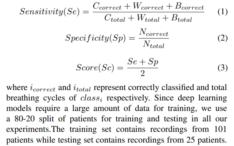
\ For a more complete evaluation of the proposed model, we also evaluate it using other commonly used metrics such as precision, recall and f1-score. Moreover, the dataset has disproportionate number of normal vs anomalous samples and the official metrics are micro-averaged (calculated over all the classes).Therefore, there is a chance that performance of the models on one class overshadows the other classes in overall results. Therefore, we calculated the precision, recall and f1- score using macro-averaging (metrics are computed for each class individually and then averaged).

\

C. Related Work

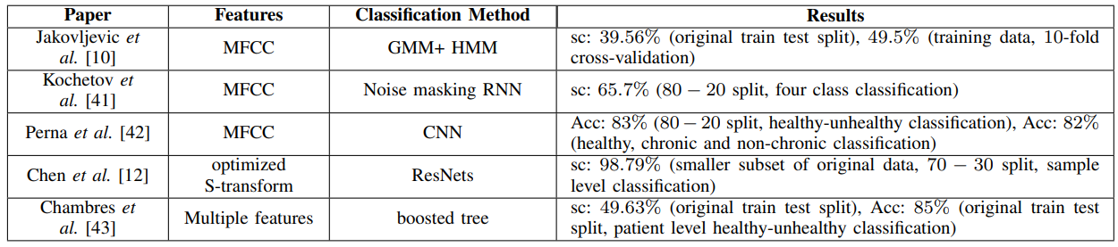
A number of papers have been published so far analyzing this dataset. Jakovljevic et al [10] used hidden markov model with Gaussian mixture model to classify the breathing cycles. They have used spectral subtraction based noise suppression to pre-process the data and MFCC features are used for classification. Their models obtained a score of 39.56% on the original train-test split and 49.5% on 10-fold cross-validation of the training set.

\ Kochetov et al. [41] proposed a noise marking RNN for the four-class classification. Their proposed model contains two sections: an attention network for binary classification of respiratory cycles into noisy and non-noisy classes and an RNN for four class classification. The attention network learns to identify noisy parts of the audio and suppress those sections and passes the filtered audio to the RNN for classifications. With a 80-20 split, they obtained a score of 65.7%. They didn’t report the score for the original train-test split. Though this method reports relatively higher scores, one primary issue with this method is that there are no noise labels in the metadata of the ICBHI dataset and the paper doesn’t mention any method for obtaining these labels. Since there are no known objective methods to measure the noise labels in these type of audio signals, this kind of manual labeling of the respiratory cycles makes their results unreliable and irreproducible.

\ Perna et al. [42] used a deep CNN architecture to classify the breathing cycles into healthy and unhealthy and obtained an accuracy of 83% using a 80-20 train-test split and MFCC features. They also did a ternary classification of the recordings into healthy,chronic and non-chronic diseases and obtained an accuracy of 82%.

\ Chen et al. [12] used optimized S-transform based feature maps along with deep residual nets (ResNets) on a smaller subset of the dataset (489 recordings) to classify the samples (not individual breathing cycles) into three classes (N, C and W) and obtained an accuracy of 98.79% on a 70-30 train-test split.

\ Finally, Chambres et al. [43] have proposed a patient level model where they classify the individual breathing cycles into one of the four classes using lowlevel features (melbands, mfcc, etc), rythm features (loudness, bpm etc), the SFX features (harmonicity and inharmonicity information) and the tonal features (chords strength, tuning frequency etc). They used boosted tree method for the classification. Next, they classified the patients as healthy or unhealthy based on the percentage of breathing cycles of the patient classified as abnormal. They have obtained an accuracy of 49.63% on the breathing cycle level classification and an accuracy of 85% on patient level classification. The justification for this patient level model is that medical professionals do not take decisions about patients based on individual breathing cycles but rather based on longer breathing sound segments and the trends represented by several breathing cycles of a patient can provide a more consistent diagnosis. A summary of the literature is presented in table I.

\

D. Proposed Method

1) Feature Extraction and Data augmentation: Since the audio samples in the dataset had different sampling frequencies, first all of the signals were down-sampled to 4kHz. Since both wheeze and crackle signals are typically present within frequency range 0 − 2kHz, down-sampling the audio samples to 4kHz should not cause any loss of relevant information.

\ As the dataset is relatively small for training a deep learning model, we used several data augmentation techniques to increase the size of the dataset. We used noise addition, speed variation, random shifting, pitch shift etc to create augmented samples. Aside from increasing the dataset size, these data augmentation methods also help the network learn useful data representations in-spite of different recording conditions, different equipments, patient age and gender, inter-patient variability of breathing rate etc.

\ For feature extraction we have used Mel-frequency spectrogram with a window size of 60 ms with 50% overlap. Each breathing cycle is converted to a 2D image where rows correspond to frequencies in Mel scale and columns correspond to time (window) and each value represent log amplitude value of the signal corresponding to that frequency and time window.

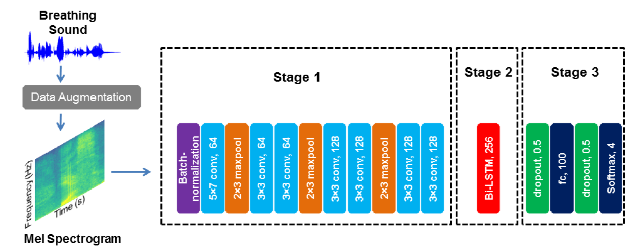
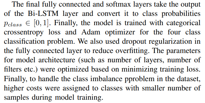
\ 2) Hybrid CNN-RNN: We propose a hybrid CNN-RNN model (figure 1) that consists of three stages: the first stage is a deep CNN model that extracts abstract feature representations from the input data, the second stage consists of a bidirectional long short term memory layer (Bi-LSTM) that learns temporal relations and finally in the third stage we have fully connected and softmax layers that convert the output of previous layers to class prediction. While these type of hybrid CNN-RNN architectures have been more commonly used in sound event detection ([44], [45]), due to sporadic nature of wheeze and crackle as well as their temporal and frequency variance, similar hybrid architectures may prove useful for lung sound classification.

\ The first stage consists of batch-normalization, convolution and max-pool layers. The batch normalization layer scales the input images over each batch to stabilize the training. In the 2D convolution layer the input is convolved with 2D kernels to produce abstract feature maps. Each convolution layer is followed by Rectified Linear activation functions (ReLU). The max-pool layer selects the maximum values from a pixel neighborhood which reduces the overall network parameters and results in shift-invariance [13].

\ LSTM have been proposed by Hochreiter and Schmidhuber [46] consisting of gated recurrent cells that block or pass the data in a sequence or time series by learning the perceived importance of data points. Each current output and the hidden state of a cell is a function of current as well as past values of the data. Bidirectional LSTM consists of two interconnected LSTM layers, one of which operates on the same direction as data sequence while the other operates on the reverse direction. So, the current output of the Bi-LSTM layer is function of current, past and future values of the data. We used tanh as non-linear activation function for this layer.

\

\ To benchmark the performance of our proposed model, we compare it to two standard CNN models, VGG-16 [40] and Mobilenet [37]. Since our dataset size is limited even after data augmentation, it can cause overfitting if we train these models from scratch on our dataset. Hence, we used Imagenet trained weights instead and replaced the dense layers of these models with an architecture similar to the fully connected and softmax layers of our proposed CNN-RNN architecture. Then the models are trained with a small learning rate.

\

\

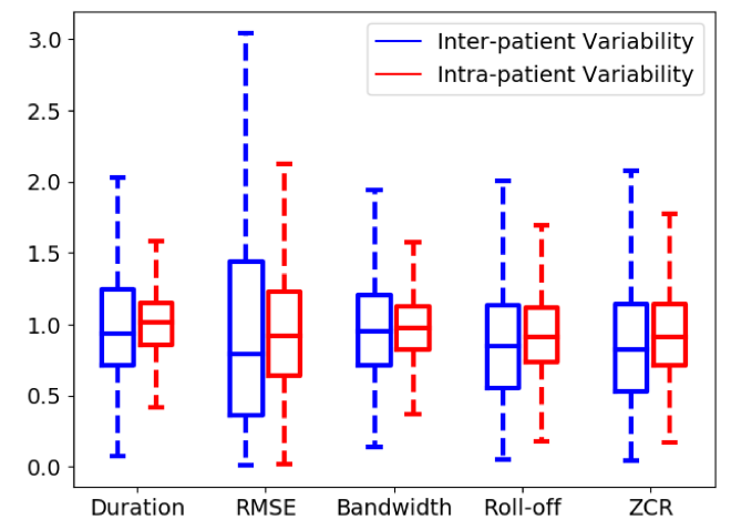
\ 3) Patient Specific Model Tuning: Though most of the existing research concentrate on developing generalized models for classifying respiratory anomalies, the problem with this kind of models is that their performance can often deteriorate for a completely new patient due to inter-patient variability. This kind of inconsistent performance of classification models make them unreliable and thus hinders their wide scale adoption. To qualitatively evaluate the inter-patient variability, we show the boxplot of inter-patient and intra-patient variability of a diverse set of audio features (duration, RMSE, bandwidth, Roll-off, ZCR) in fig. 2. For the intra-patient variability, we normalized each audio feature of a sample by average of that feature for the samples from that specific patient while for inter-patient variability, we normalized the audio features by the average of that feature over the entire dataset. As evident from the figure, inter-patient variability is significantly larger when compared to intra-patient variability.

\ Also, from a medical professional’s perspective, for most of the chronic respiratory patients, some patient data is already available or can be collected and automated long-term monitoring of patient condition after initial treatment is often very important. Though training a model based on existing patient specific data to extract patient specific features result in a more consistent and reliable patient specific model, it is often very difficult to collect enough data from a patient to sufficiently train a machine learning model. Since deep learning models require much larger amount of data for training, the issue is further exacerbated.

\ To address these shortcomings of existing methods, we propose a patient specific model tuning strategy that can take advantage of deep learning techniques even with small amount of patient data available. In this proposed model, the deep network is first trained on a large database to learn domain specific feature representations. Then a smaller part of the network is re-trained on the small amount of patient specific data available. This enables us to transfer the learned domain specific knowledge of the deep network to patient specific models and thus produce consistent patient specific class predictions with high accuracy. In our proposed model we train the 3 stage network on the training samples. Then, for a new patient, only the last stage is re-trained with patient specific breathing cycles while the learned CNN-RNN stage weights are frozen in their pre-trained values. For our proposed strategy only ∼ 1.4% of the network parameters are retrained for patient specific models. For VGG-16 and MobileNet, the same strategy is applied.

\ 4) Weight Quantization: In this proposed weight quantization scheme, the magnitude of weights of each layer are quantized in log domain. The quantized weight (w˜) can be represented as:

\

\

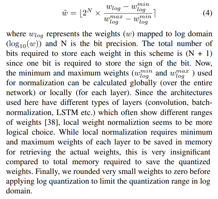
:::info Authors:

(1) Jyotibdha Acharya (Student Member, IEEE), HealthTech NTU, Interdisciplinary Graduate Program, Nanyang Technological University, Singapore;

(2) Arindam Basu (Senior Member, IEEE), School of Electrical and Electronic Engineering, Nanyang Technological University, Singapore.

:::

:::info This paper is available on arxiv under ATTRIBUTION-NONCOMMERCIAL-SHAREALIKE 4.0 INTERNATIONAL license.

:::

\