Can Math Fix Uniswap v3 LP Losses? New Strategy Says Yes, but With a Catch
Table Of Links
Abstract
1. Introduction
2. Constant function markets and concentrated liquidity
- Constant function markets
- Concentrated liquidity market
3. The wealth of liquidity providers in CL pools
- Position value
- Fee income
- Fee income: pool fee rate
- Fee income: spread and concentration risk
- Fee income: drift and asymmetry
- Rebalancing costs and gas fees
4. Optimal liquidity provision in CL pools
- The problem
- The optimal strategy
- Discussion: profitability, PL, and concentration risk
- Discussion: drift and position skew
5. Performance of strategy
- Methodology
- Benchmark
- Performance results
6. Discussion: modelling assumptions
- Discussion: related work
7. Conclusions And References
\
Performance Of Strategy
5.1. Methodology
In this section, we use Uniswap v3 data between 1 January and 18 August 2022 (see data description in Appendix A) to study the performance of the strategy of Section 4. We consider execution costs and discuss how gas fees and liquidity taking activity in the pool affect the performance of the strategy.13
\ Our strategy in Section 4 is solved in continuous time. In our performance study, we discretise the trading window in one-minute periods and the optimal spread is fixed at the beginning of each time-step. That is, let ti be the times where the LP interacts with the pool, where i ∈ {1, . . . , N} and ti+1 − ti = 1 minute. For each time ti , the LP uses the optimal strategy in (27) based on information available at time ti , and she fixes the optimal spread of her position throughout the period [ti , ti+1); recall that the optimal spread is not a function of time.
\ To determine the optimal spread (27) of the LP’s position at time ti , we use in-sample data [ti − 1 day, ti ] to estimate the parameters. The volatility σ of the rate Z is given by the standard deviation of one-minute log returns of the rate Z, which is multiplied by √ 1440 to obtain a daily estimate. The pool fee rate πt is given by the total fee income generated by the pool during the insample period, divided by the pool size 2 κ Z1/2 t at time t, where κ is the active depth at time t.
\ We run the linear regression described in Section 3.2.2 to estimate the concentration cost parameter, which is set to γ = 5 × 10⁻⁷ . Finally, prediction of the future marginal rate Z is out of the scope of this work, thus we set µ = 0 and ρ = 0.5. To compute the LP’s performance as a result of changes in the value of her holdings in the pool (position value), and as a result of fee income, we use out-of-sample data [ti , ti+1].
\ We use equation (9) to determine the one-minute out-of-sample changes in the position value. For fee income, we use LT transactions in the pool at rates included in the range Z ℓ t , Zu t and equation (4). The income from fees accumulates in a separate account in units of X with zero risk-free rate.14 At the end of the out-of-sample window, the LP withdraws her liquidity and collects the accumulated fees, and we repeat the in-sample estimation and out-of-sample liquidity provision described above.
\ Thus, at times ti , where i ∈ {1, . . . , N −1}, the LP consecutively withdraws and deposits liquidity in different ranges. Between two consecutive operations (i.e., reposition liquidity provision), the LP may need to take liquidity in the pool to adjust her holdings in asset X and Y. In that case, we use results in Cartea et al. (2022) to compute execution costs.15 In particular, we consider execution costs when the LP trades asset Y in the pool to adjust her holdings between two consecutive operations.
\ More precisely, we consider that for every quantity y of asset Y bought or sold in the pool, a transaction cost y Z3/2 t /κ is incurred. We assume that the LP’s taking activity does not impact the dynamics of the pool. Finally, we obtain 331,858 individual LP operations from 1 January to 18 August 2022.
\ 5.2. Benchmark
We compare the performance of our strategy with the performance of LPs in the pool we consider. We select operation pairs that consist of first providing and then withdrawing the same depth of liquidity κ˜ at two different points in time by the same LP.16 The operations that we select represent approximately 66% of all LP operations. Figure 9 shows the distribution of key variables that describe how LPs provide liquidity.
\ The figure shows the distribution of the number of operations per LP, the changes in the position value, the length of time the position is held in the pool, and the position spread. Finally, Table 2 shows the average and standard deviation of the distributions in Figure 9. Notice that the bulk of liquidity is deposited in small ranges, and positions are held for short
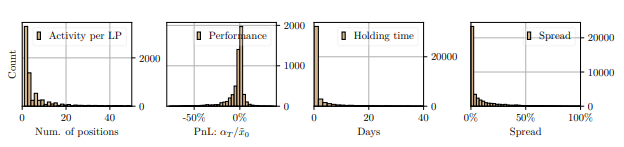 periods of time; 20% of LP positions are held for less than five minutes and 30% for less than one hour. Table 2 also shows that, on average, the performance of the LP operations in the pool and the period we consider is −1.49 % per operation.
\ 5.3. Performance results
This subsection focuses on the performance of our strategy when gas fees are zero — at the end of the section we discuss the profitability of the strategy when gas fees are included. Figure 10 shows the distribution of the optimal spread (24) posted by the LP. The bulk of liquidity is deposited in ranges with a spread δ below 1%.
\ Table 2 compares the average performance of the components of the optimal strategy with the performance of LP operations observed in the ETH/USDC pool.17 Table 3 suggests that the position of the LP loses value in the pool (on average) because of PL; however, the fee income would cover the loss, on average, if one assumes that gas fees are zero. Finally, the results show that our optimal strategy significantly improves the PnL of LP activity in the pool and the performance of the assets themselves.
The results in Table 3 do not consider gas fees. Gas cost is a flat fee, so it does not depend on the position spread or size of transaction. If the activity of the LP does not affect the pool and if the fees collected scale with the wealth that the LP deposits in the pool, then the LP should consider an initial amount of X and Y that would yield enough fees to cover the flat gas fees.
\ An estimate of the average gas cost gives an estimate of the minimum amount of initial wealth for a self-financing strategy to be profitable. Recall that, at any point in time t, the LP withdraws her liquidity, adjusts her holdings, and then deposits new liquidity. In the data we consider, the average gas fee is 30.7 USD to provide liquidity, 24.5 USD to withdraw liquidity, and 29.6 USD to take liquidity.
\ Average gas costs are obtained from blockchain data which record the gas used for every transaction, and from historical gas prices. The LP pays a flat fee of 84.8 USD per operation when implementing the strategy in the pool we consider, so the LP strategy is profitable, on average, if the initial wealth deposited in the pool is greater than 1.8 × 10⁶ USD.
\ Fee income of the LP strategy is limited by the volume of liquidity taking activity in the pool, so one should not only consider increasing the initial wealth to make the strategy more profitable. There are 4.7 LT transactions per minute and the average volume of LT transactions is 477, 275 USD per minute, so if the LP were to provide 100% of the liquidity, the average fee income per operation would be 1,431 USD.
:::info Authors:
- Alvaro Cartea ´
- Fayc¸al Drissia
- Marcello Monga
:::
:::info This paper is available on arxiv under CC0 1.0 Universal license.
:::
\


You May Also Like

Leap Wallet to Shut Down by May 28 as Team Winds Down Apps and Validator
Crypto Sectors Reveal Striking Divergence: 5 Explosive Gainers and 5 Troubled Decliners in 2025